Sketching the Graph of a function II

Truth is not what you want it to be; it is what it is. And you must bend to its power or live a lie, Miyamoto Musashi.

The truth is multifaceted and complex. Life is always messier than our dreams and beliefs, reality is more complicated that we think it is, it is constantly changing like the wind and the future is not promised, but completely unpredictable, JustToThePoint, Anawim, #justtothepoint.

Recall

Definition. A function f is a rule, relationship, or correspondence that assigns to each element of one set (x ∈ D), called the domain, exactly one element of a second set, called the range (y ∈ E).

The pair (x, y) is denoted as y = f(x). Typically, the sets D and E will be both the set of real numbers, ℝ.

Graphing functions involves the visual representation of a curve that reflects the behavior of a mathematical function on a coordinate plane, also known as the Cartesian plane. It is a two-dimensional space defined by two axes - the x-axis (horizontal) and the y-axis (vertical).

A systematic approach to graphing a function begins by constructing a table containing selected input values and their corresponding output values. By extending this table, we can plot the points on the coordinate plane and observe the pattern they form. Connecting these points reveals the shape of the curve, allowing us to gain insights into the behavior of the function across its domain. This process provides a visual means of understanding the relationships between different variables and aids in interpreting the overall characteristics of the function.

General strategy to plot functions

1. Find undefined values and the function's domain.
2. Locate discontinuities and the x- and y-intercepts.
3. Study the end behavior, determine whether f has any horizontal, vertical, or oblique asymptotes.
4. Check for symmetries. This can immensely reduce the amount of work you need to do.
5. Calculate f’. Solve f’(x) = 0. Plot easy points, critical points, and determine the intervals where f is increasing or decreasing.
6. Determine whether f has any local extrema, i.e., minimums or maximums.
7. Calculate f’’. Determine the intervals where f is concave up or down, and its inflection points.

Basic Transformations

Sometimes we draw the parent graph and then apply the relevant transformation to the graph:

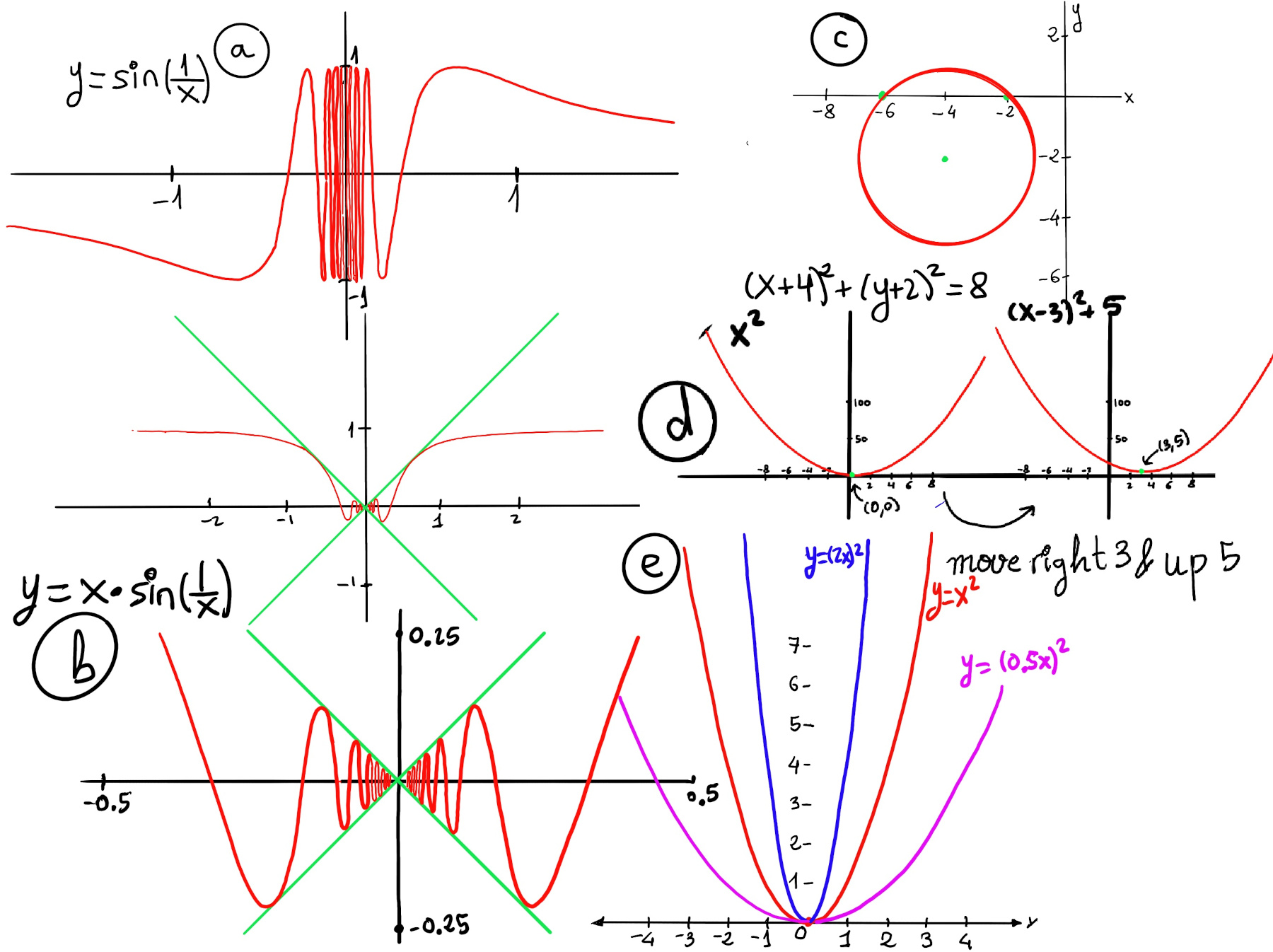
1. A translation of a function is a shift in one or more directions. It is a transformation that moves the function’s graph horizontally or vertically without changing its shape. f(x) + a shifts the graph vertically “a” units, f(x + a) shifts the graphs horizontally by “a” units, e.g., (x -3)² + 5 (Figure d) moves x² three unit to the right and five units up.

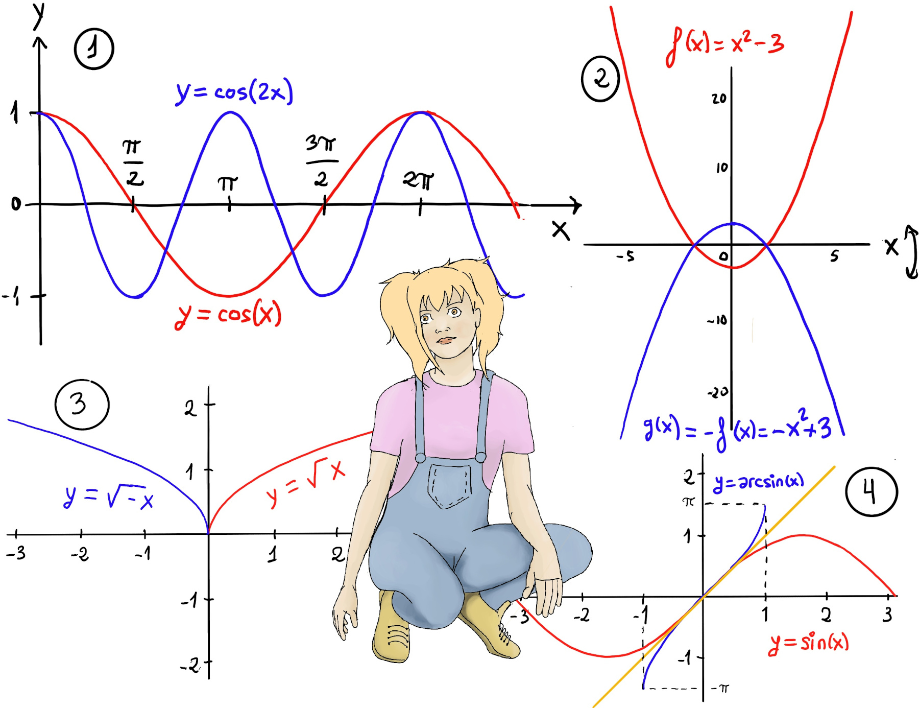
2. f(ax) where |a| > 1 squeezes or compresses the graph toward the y-axis, e.g., y = (2x)² (Figure e), y = cos(2x) (Figure 1). Conversely, f(ax) where 0 < |a| < 1 dilates the graph toward the y-axis, causing all points to move away from the axis to a multiple of their original distance from the axis e.g., y = (0.5x)² (Figure e).

    

    

   The function 4(x -2)² +3 has a simpler “parent” function f(x) = x². f has been dilated vertically by a factor of 4, then translated vertically by +3 and horizontally by 2 to produce our original function.

3. A reflection is a transformation where a curve is flipped in a line of reflection. -f(x) is a reflection in the x-axis, e.g., f(x) = x² -3, g(x) = -f(x) = -x² +3. f(-x) is a reflection in the y-axis (Figure 2). f(-x) is a reflection in the y-axis, e.g., f(x) = $\sqrt{x}$, Domain(f) = ℝ⁺, g(x) = f(-x) = $\sqrt{-x}$ (Figure 3), Domain(g) = ℝ⁻.

Plotting Piecewise functions

Piecewise functions. We can create functions that behave differently based on the input (x) value. It is a function that defines different expressions for different intervals of the domain. Plotting these functions involves graphing different parts of the function for different intervals of the domain based on the conditions specified by their definition.

• Let $f(x) = \begin{cases} -x + 2, &x < 0 \\ x^2 + 2, &x ≥ 0 \end{cases}$

Approaching 0 from the left (x < 0), f(x) becomes -x + 2 and as we get closer and closer to 2, $\lim_{x \to 0⁻} f(x) = \lim_{x \to 0⁻} -x + 2 = 2$. Approaching 0 from the right (x > 0), f(x) becomes x² + 2 and as we get closer and closer to 2, $\lim_{x \to 0⁺} f(x) = \lim_{x \to 0⁺} x^2 + 2 = 2.$

Therefore, $\lim_{x \to 0} f(x)$ = 2, (Figure i).

• Let $f(x) = \begin{cases} 2x + 1, &x < -5 \\ x^2 -12, &x > -5 \end{cases}$

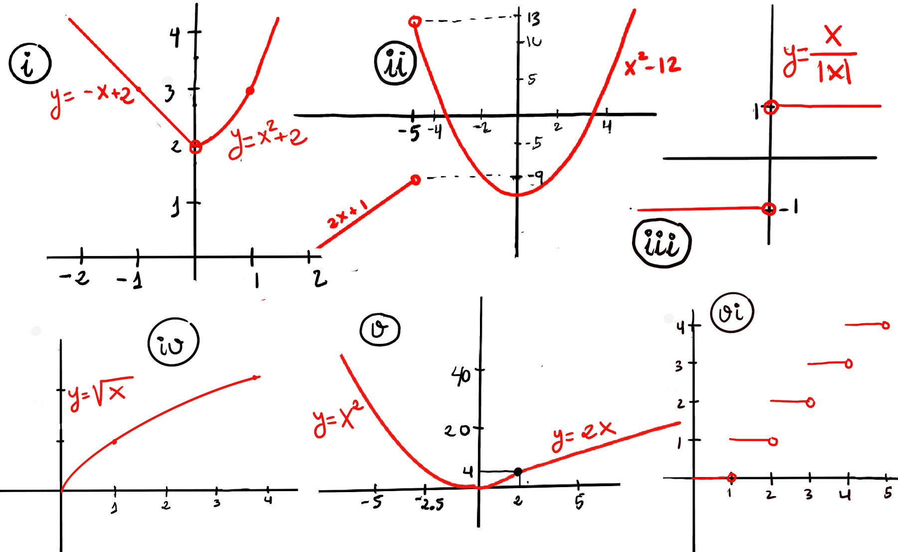
Approaching -5 from the left (x < -5), f(x) becomes 2x + 1 and as we get closer and closer to -5, $\lim_{x \to -5⁻} f(x) = \lim_{x \to -5⁻} 2x +1 = 2·-5 + 1 = -9$. Approaching -5 from the right (x > -5), f(x) becomes x²-12 and as we get closer and closer to -5, $\lim_{x \to -5⁺} f(x) = \lim_{x \to -5⁺} x^2 -12 = (-5)^2 -12 = 25 -12 = 13$.

Therefore, $\lim_{x \to -5} f(x)$ does not exist because the left and right limits are different, (Figure ii).

• Let $f(x) = \frac{|x|}{x} = \begin{cases} -1, &x < 0 \\ 1, &x > 0 \end{cases}$

$\lim_{x \to 0} \frac{|x|}{x}$. Notice that $\frac{|x|}{x}$ is not defined at x = 0. $\lim_{x \to 0⁻} f(x) = \lim_{x \to 0⁻} \frac{-x}{x} = -1, \lim_{x \to 0⁺} f(x) = \lim_{x \to 0⁺} \frac{x}{x} = 1$, hence $\lim_{x \to 0} \frac{|x|}{x}$ does not exist (figure iii).

Figure iv, v, and vi are the corresponding plots of $f(x)=\sqrt{x}$, Domain(f) = ℝ⁺, $f(x) = \begin{cases} x^2, &x < 2 \\ 2x, &x ≥ 2 \end{cases}$, and the greatest integer function ⌊x⌋ (More information at One sided limits).

Plotting inverse functions

Loosely speaking, the inverse function of a function f is a function that undoes the operation of the original function. If f is a function that maps each element x in its domain to a unique element y in its codomain, then the inverse function, denoted as $f^{-1}$, maps each element y back to its corresponding x.

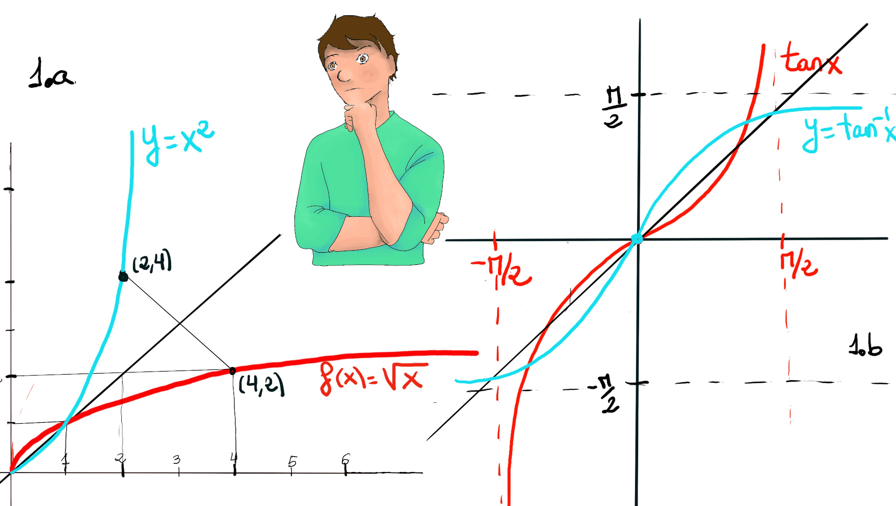
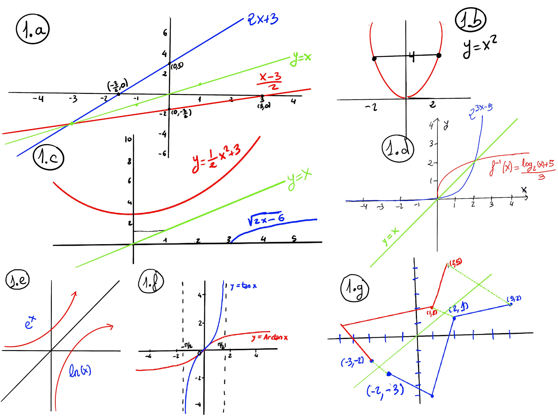
For a given function f, its inverse g(=f^-1) is a function that reverses its result (g reverses the input and output of the original function), g(f(x))=x. An example is f(x)=$\sqrt{x},$ (x ≥ 0) g(f(x))=x ↭ g(x)= x², -1.a.- The square function (x²) is the inverse of the square root function ($\sqrt{x}$). The natural logarithm function is the inverse of the exponential function (1.e.). Logarithmic functions are the inverses of exponential functions, y = a^x, f^-1(x) = log_a(x).

If you want to plot the graph of f^-1, you just need to reflect the graph of f(x) about the line y = x.  

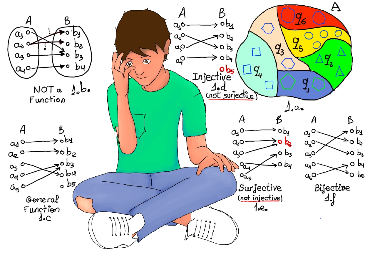
For an inverse function to exist, the original function must be both one-to-one (injective) and onto (surjective). A function is one-to-one if each element of the domain maps to a distinct (unique) element in the codomain, and it is onto if every element in the codomain is mapped to by at least one element in the domain or, in other words, has a pre-image in the domain.

Some examples are shown in the below figure, f(x) = 2x + 3 ↭ f^-1(x) = $\frac{x-3}{2}$ (Figure 1.a), f(x) = $\frac{1}{2}x^2+3, f^{-1}(x)=\sqrt{2x-6}$ (Figure 1.c), f(x) = $2^{3x-5}, f^{-1}(x)=\frac{log_2(x)+5}{3}$ (Figure 1.d), f(x) = $e^x, f^{-1}(x)=ln(x)$ (Figure 1.e, Exponential functions, Logarithm functions), and f(x) = $tan(x), f^{-1}(x)=arctan(x)$ (Figure 1.f).

Solved examples

• $\frac{x^{2}}{1-x^{2}}$

1. Domain = ℝ - {1, -1}. f(0) = 0.
2. f(-x)=f(x), so this function is even.
3. $\lim_{x \to \pm\infty}\frac{x^{2}}{1-x^{2}}=-1$, y = -1 is a horizontal asymptote.
4. $\lim_{x \to 1^{+}}\frac{x^{2}}{1-x^{2}}=\frac{1}{0^{-}} = -\infty, \lim_{x \to 1^{-}}\frac{x^{2}}{1-x^{2}}=\frac{1}{0^{+}} = \infty$. Similarly, $\lim_{x \to -1^{+}}\frac{x^{2}}{1-x^{2}}=\frac{1}{0^{+}} = \infty, \lim_{x \to -1^{-}}\frac{x^{2}}{1-x^{2}}=\frac{1}{0^{-}} = -\infty$, hence x = -1 and x = 1 are vertical asymptotes.
5. f’(x) = $\frac{2x}{(1-x^{2})^{2}}$. Critical points: 0 (f’(x)=0), 1 and -1 (f’ is undefined). x < -1, f’(x) < 0 ⇒ f decreasing ↘. -1 < x < 0, f’(x) < 0 ⇒ f decreasing ↘. 0 < x < 1, f’(x) > 0 ⇒ f increasing ↗. x > 1, f’(x) > 0 ⇒ f increasing ↗.
6. f’’(x) = $\frac{6x^{2}+2}{(1-x^{2})^{3}}$. x < -1, f’’(x) < 0 ⇒ concave downward
   -1 < x < 1, f’’(x) > 0 ⇒ concave upward
   x > 1, f’’(x) < 0 ⇒ concave downward

The plot is shown in Figure 1.d.  

• f(x) = ^x⁄_lnx, x > 0.

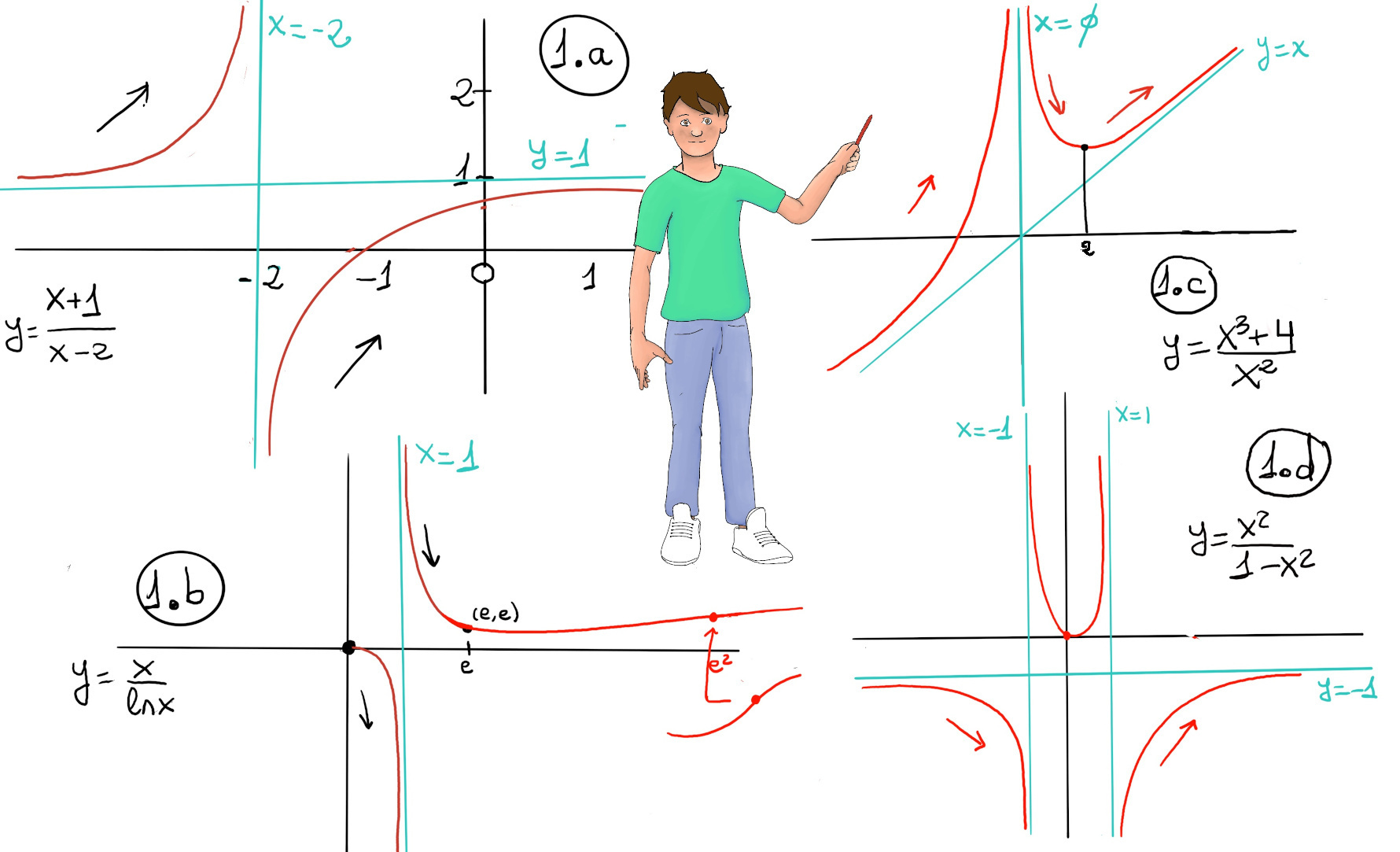
There is another undefined value x = 1, Dom(f) = ℝ⁺ - {0, 1}, and $\lim_{x \to 1^{+}}\frac{x}{lnx}=\frac{1}{0^{+}}=\infty, \lim_{x \to 1^{-}}\frac{x}{lnx}=\frac{1}{0^{-}}=-\infty$. Therefore, x = 1 is a vertical asymptote.

Let’s study the end behavior: $\lim_{x \to 0^{+}}\frac{x}{lnx}=\frac{0}{-\infty}=\lim_{x \to 0^{+}} {\frac{1}{\frac{1}{x}}}= \lim_{x \to 0^{+}}x = 0, \lim_{x \to \infty}\frac{x}{lnx}=~ -L’Hopitals Rule-~\lim_{x \to \infty} {\frac{1}{\frac{1}{x}}}= \lim_{x \to \infty}x = \infty$

f’(x) = $\frac{lnx-x(\frac{1}{x})}{(lnx)^{2}}=~ \frac{lnx -1}{(lnx)^{2}}$

f’(x) = 0 ↭ lnx = 1 ↭ x = e, and f(e) = e.

Futhermore: If 0 < x < 1, f’(x) < 0 ⇒ f is decreasing ↘. 1 < x < e, f’(x) < 0 ⇒ f is decreasing ↘. x > e, f’(x) > 0 ⇒ f is increasing ↗. Hence, f has a local minimum at x = e.

Let’s calculate f’’(x) = $\frac{\frac{1}{x}(lnx)^{2}-\frac{(lnx-1)2lnx}{x}}{(lnx)^{4}}=~ \frac{\frac{lnx-2(lnx-1)}{x}}{(lnx)^{3}}=~ \frac{2-lnx}{x(lnx)^{3}}$

Therefore, 0 < x < 1, f’’(x) < 0 ⇒ concave down. 1 < x < e², f’(x) > 0 ⇒ concave up. x > e², f’(x) < 0 ⇒ concave down. Therefore, e² is an inflection point, a point where concavity changes. The plot is shown in Figure 1.b.  

Some exotic examples

• y = $sin(\frac{1}{x})$

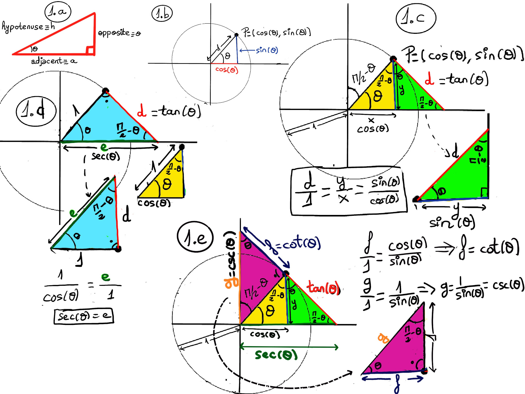
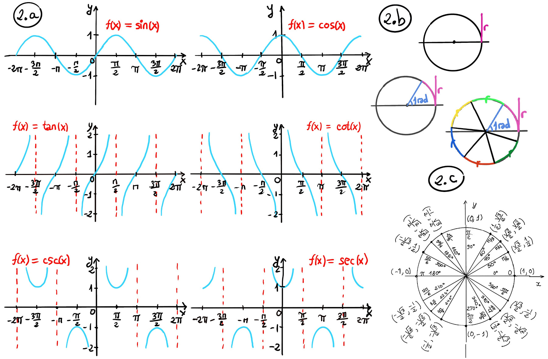
The sine function is the ratio of the length opposite to the given angle and the hypotenuse of the given triangle, $sin(θ) = \frac{opposite}{hypotenuse} = \frac{o}{h}$. It is odd (sin(-x) = -sin(x), the graph is symmetric with respect to the origin), periodic with a period of 2π, and it ranges between -1 and 1 (Figures 1.a. and 2.a.).

It is essential to notice that $|sin(\frac{1}{x})| ≤ 1,$ hence the graph is bounded by y = -1 and y = 1. The zeros are precisely x = $\frac{1}{πn}$. As x approaches 0, the reciprocal term becomes very large, causing the sine function to oscillate rapidly between -1 and 1. Besides, it is not defined at x = 0, and it does not have a limit at x = 0 (Figure a).

• y = $x·sin(\frac{1}{x})$ (Figure b).

Recall that $|sin(\frac{1}{x})| ≤ 1 ↭ -1 ≤ sin(\frac{1}{x}) ≤ 1 ⇒ -x ≤ x·sin(\frac{1}{x}) ≤ x$ meaning that the graph is bounded by y = x and y = -x, and because of the squeeze theorem, $\lim_{x \to 0} x·sin(\frac{1}{x}) = 0$.

Near x = 0, both the sinusoidal and reciprocal part ensure rapid oscillations bounded between the graphs of y =x and y = -x.

$\lim_{x \to ∞} x·sin(\frac{1}{x}) = \lim_{x \to ∞} \frac{sin(\frac{1}{x})}{\frac{1}{x}} = \lim_{x \to ∞} \frac{cos(\frac{1}{x})·\frac{-1}{x^2}}{\frac{-1}{x^2}} = \lim_{x \to ∞} cos(\frac{1}{x}) = cos(0) = 1$, so moving away from the origin, someone near x = ±1, it will touch y = ±x for the last time, and then asymptotically approach y = 1.

Bibliography

1. NPTEL-NOC IITM, Introduction to Galois Theory.
2. Algebra, Second Edition, by Michael Artin.
3. LibreTexts, Calculus.
4. Field and Galois Theory, by Patrick Morandi. Springer.
5. Michael Penn, and MathMajor.
6. Contemporary Abstract Algebra, Joseph, A. Gallian.
7. YouTube’s Andrew Misseldine: Calculus, College Algebra and Abstract Algebra.
8. Calculus Early Transcendentals: Differential & Multi-Variable Calculus for Social Sciences.
9. blackpenredpen.