Asymptotes and End Behavior

Recall

Definition. A function f is a rule, relationship, or correspondence that assigns to each element of one set (x ∈ D), called the domain, exactly one element of a second set, called the range (y ∈ E).

The pair (x, y) is denoted as y = f(x). Typically, the sets D and E will be both the set of real numbers, ℝ.

Graphing functions involves the visual representation of a curve that reflects the behavior of a mathematical function on a coordinate plane, also known as the Cartesian plane. It is a two-dimensional space defined by two axes - the x-axis (horizontal) and the y-axis (vertical).

A systematic approach to graphing a function begins by constructing a table containing selected input values and their corresponding output values. By extending this table, we can plot the points on the coordinate plane and observe the pattern they form. Connecting these points reveals the shape of the curve, allowing us to gain insights into the behavior of the function across its domain. This process provides a visual means of understanding the relationships between different variables and aids in interpreting the overall characteristics of the function.

Asymptotes and End Behavior of Functions

An asymptote is a horizontal, vertical, or slanted line such that the distance between the graph and the line approaches zero as one or both of the x or y coordinates tends to infinity. In other words, it is a line that the graph approaches (it gets closer and closer, but never quite reach) as it heads or goes to positive or negative infinity.

Vertical asymptotes are vertical lines (perpendicular to the x-axis) of the form x = a (where a is a constant) near which the function grows without bound. The line x = a is a vertical asymptote if: $\lim_{x \to a^{-}}f(x)=\pm\infty$ or $\lim_{x \to a^{+}}f(x)=\pm\infty$, e.g., x = -2 is a vertical asymptote of $\frac{x+1}{x+2}$.

$\lim_{x \to -2^{+}}\frac{x+1}{x+2} = \frac{-1}{0⁻} = \infty, \lim_{x \to -2^{-}}\frac{x+1}{x+2} = \frac{-1}{0⁺} = -\infty$

Horizontal asymptotes are a means of describing end behavior of functions and very closely related to limits at infinity. Horizontal asymptotes are horizontal lines (parallel to the x-axis) that the graph of the function approaches as x → ±∞. y = c is a horizontal asymptote if the function f(x) becomes arbitrarily close to c as long as x is sufficiently large or small or more formally: $\lim_{x \to \infty}f(x)=c$ and/or $\lim_{x \to -\infty}f(x)=c$, e.g., y = 1 is a horizontal asymptote of $\frac{x+1}{x+2}$ because $\lim_{x \to \pm\infty}\frac{x+1}{x+2} = 1$.

A polynomial is a function of the form f(x) = a_nxⁿ + a_n-1xⁿ⁻¹ + … + a₂x² + a₁x + a₀. The degree of a polynomial is the highest power of x in its expression. Polynomial functions are defined and continuous on all real numbers. The degree and the leading coefficient of a polynomial determine the end behavior of its graph.

 

Rational Functions

Definition. Rational functions are ratios of two polynomial functions, f(x) = $\frac{p(x)}{q(x)} = \frac{a_nx^n+a_{n−1}x^{n−1}+…+a_1x+a_0}{b_mx^m+b_{m−1}x^{m−1}+…+b_1x+b_0}$ where a_n ≠ 0, b_m ≠ 0, and q(x) ≠ 0, e.g., $\frac{3-2x}{x-2}, \frac{x^3 + x^2 - 2x + 12}{x+3}.$

The limits at infinity for a rational function, say f(x) = $\frac{p(x)}{q(x)} = \frac{a_nx^n+a_{n−1}x^{n−1}+…+a_1x+a_0}{b_mx^m+b_{m−1}x^{m−1}+…+b_1x+b_0}$, can be exclusively determined or calculated based on its degrees (Limits of Rational Functions):

• The degree of the numerator and the denominator are the same, $\lim_{x \to ∞} f(x) = \lim_{x \to ∞} \frac{a_nx^n+a_{n−1}x^{n−1}+…+a_1x+a_0}{b_mx^m+b_{m−1}x^{m−1}+…+b_1x+b_0} = \frac{a_n}{b_m}$ where m = n, a_n and b_n = b_m are the leading coefficients of p and q respectively. The line $ y = \frac{a_n}{b_m}$ is a horizontal asymptote, e.g., $\lim_{x \to ∞} \frac{2x^7+4x^3+2x+1}{3x^7+4x^2+3x+5} = \frac{2}{3}, \lim_{x \to ∞} \frac{4x^2+2x+7}{3x^2+3x+2} = \frac{4}{3}, \lim_{x \to ∞} \frac{2x^5+3x^4+2x^3+7x+1}{2x^5+12x^4+3x^2+2x+8} = 1.$
• The degree of the numerator is smaller than the degree of the denominator, $\lim_{x \to ∞} f(x) = \lim_{x \to ∞} \frac{a_nx^n+a_{n−1}x^{n−1}+…+a_1x+a_0}{b_mx^m+b_{m−1}x^{m−1}+…+b_1x+b_0} = 0$. The line y = 0 is a horizontal asymptote, e.g., $\lim_{x \to ±∞} \frac{2x^6+4x^3+2x+1}{3x^7+4x^2+3x+5} = 0, \lim_{x \to ∞} \frac{4x^2+2x+7}{3x^3+3x+2} =0, \lim_{x \to ∞} \frac{2x^5+3x^4+2x^3+7x+1}{2x^7+2x^4+3x^2+2x+8} = 0.$
• The degree of the numerator is bigger than the degree of the denominator, $\lim_{x \to ∞} f(x) = \lim_{x \to ∞} \frac{a_nx^n+a_{n−1}x^{n−1}+…+a_1x+a_0}{b_mx^m+b_{m−1}x^{m−1}+…+b_1x+b_0} = ±∞$, e.g., $\lim_{x \to ∞} \frac{2x^5+8x^2+8}{9x^3+4x^2+3x+5} = \lim_{x \to ∞} \frac{2x^5}{9x^3} = \lim_{x \to ∞} \frac{2x^2}{9} = ∞,\lim_{x \to -∞} \frac{4x^3+2x+7}{3x^2+3x+2} = \lim_{x \to -∞} \frac{4x^3}{3x^2} = \lim_{x \to -∞} \frac{4x}{3} = -∞,\lim_{x \to ∞} \frac{4x^3+2x+7}{3x^2+3x+2} = \lim_{x \to ∞} \frac{4x^3}{3x^2} = \lim_{x \to ∞} \frac{4x}{3} = ∞.$

End Behaviour of exponential functions

An exponential function is a mathematical function of the form f(x) = b·a^x, where the independent variable is the exponent, and a and b are constants. a is called the base of the function and it should be a positive real number (a>0).

1. If a > 1, it can be observed that as the exponent increases, the curve get steeper. As x increases, f(x) heads to infinity, $\lim_{x \to ∞} a^x = ∞$. As x decreases, f(x) heads to zero, $\lim_{x \to -∞} a^x = 0$. It is strictly increasing ((e^x)’ = e^x > 0, (a^x)’ = a^x·ln(a) > 0) and has a horizontal asymptote along the x-axis.

   It is important to realize that as x approaches negative infinity, the results become very small but never actually attain zero, e.g., 2^-5 ≈ 0.03125, 2^-15 ≈ 0.00003052. Besides, the base of an exponential function determines the rate of growth or decay. For a > 1, the larger the base, the faster the function grows (Figure iii).

    
2. 0 < a < 1. As x increases, f(x) heads to zero, $\lim_{x \to ∞} a^x = 0$. As x decreases, f(x) heads to ∞, $\lim_{x \to -∞} a^x = ∞$. It is strictly decreasing and has a horizontal asymptote along the x-axis.
3. When a = 1, the graph is a horizontal line, y = 1.  

End Behaviour of logarithmic functions

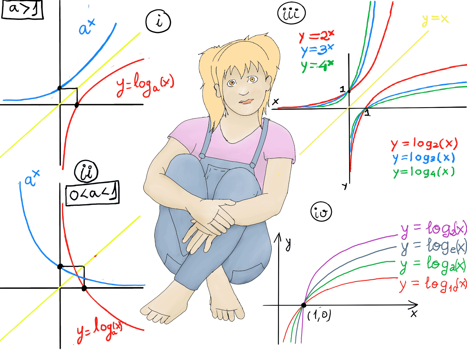
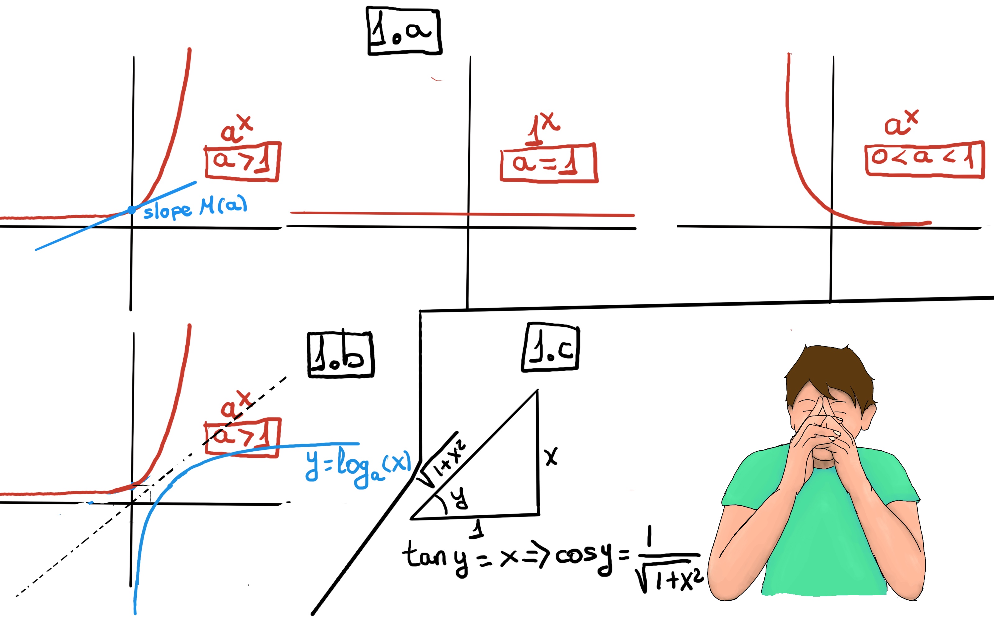
In mathematics, the logarithm is the inverse function to exponentiation. We call the inverse of a^x the logarithmic function with base a, that is, log_ax=y ↔ a^y=x, that means that the logarithm of a number x to the base a is the exponent to which a must be raised to produce x, e.g., log₄(64) = 3 ↭ 4³ = 64, log₂(16) = 4 ↭ 2⁴ = 16, log₈(512) = 3 ↭ 8³ = 512, but log₂(-3) is undefined.

The logarithm’s domain consists of real positive numbers. Its range is ℝ (figure i and ii). x-intercept: (1, 0), y-intercept: none. It is one-to-one and has a vertical asymptote along the y-axis at x = 0.

1. If a > 1, it can be observed that as the value of the argument increases, the logarithm’s value increases as well. As x increases, f(x) heads to infinity, $\lim_{x \to ∞} log_a(x) = ∞$. As x decreases, f(x) heads to zero, $\lim_{x \to 0+} log_a(x) = 0$. It is strictly increasing and has a vertical asymptote along the y-axis at x = 0.

   The bigger the logarithm base, the graph approaches the asymptote of x = 0 quicker (Figure iii and iv).

2. If 0 < a < 1, it can be observed that as the value of the argument increases, the logarithm’s value decreases. As x increases, f(x) heads to minus infinity, $\lim_{x \to ∞} log_a(x) = -∞$. As x decreases, f(x) heads to zero, $\lim_{x \to 0+} log_a(x) = 0$. It is strictly decreasing and has a vertical asymptote along the y-axis at x = 0.

Solved examples

Identify the asymptotes and end behavior of the following functions:

• $ \frac{1}{x}$ (Figure i). $\lim_{x \to 0⁺} \frac{1}{x} = +∞, \lim_{x \to 0⁻} \frac{1}{x} = -∞$ ⇒ x = 0 is a vertical asymptote. $\lim_{x \to +∞} \frac{1}{x} = \lim_{x \to -∞} \frac{1}{x}= 0$ ⇒ y = 0 or the x-axis is a horizontal asymptote.

• We don’t have an expression for (ii). There is a horizontal asymptote, y = 1. As x approaches positive and negative infinity, there is a horizontal asymptote, y = 1, even though the function clearly passes through this line an infinite number of times.  

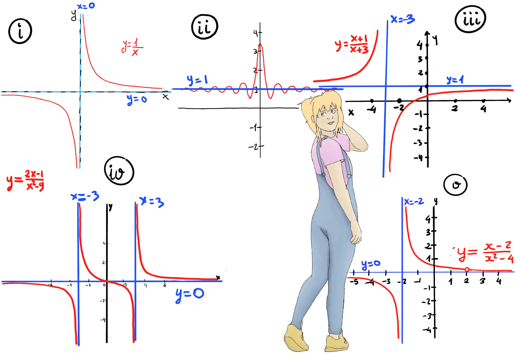
• $\frac{x+1}{x+3}$ (Figure iii). $\lim_{x \to -3⁺} \frac{x+1}{x+3} = \frac{-2}{0⁻} = ∞, \lim_{x \to -3⁻} \frac{x+1}{x+3} = = \frac{-2}{0⁺} = -∞$ ⇒ x = 3 is a vertical asymptote. $\lim_{x \to +∞} \frac{x+1}{x+3} = \lim_{x \to -∞} \frac{x+1}{x+3}= 1$ ⇒ y = 1 is a horizontal asymptote.

• $\frac{2x+1}{x^2-9}$ (Figure iv). $\lim_{x \to -3⁺} \frac{2x+1}{x^2-9} = \frac{-5}{0⁺} = -∞, \lim_{x \to -3⁻} \frac{2x+1}{x^2-9} = \frac{-5}{0⁻} = +∞$ ⇒ x = -3 is a vertical asymptote. Similarly, $\lim_{x \to 3⁺} \frac{2x+1}{x^2-9} = \frac{7}{0⁺} = +∞, \lim_{x \to 3⁻} \frac{2x+1}{x^2-9} = \frac{7}{0⁻} = -∞$ ⇒ x = 3 is a vertical asymptote, too.

$\lim_{x \to +∞} \frac{2x+1}{x^2-9} = \lim_{x \to -∞} \frac{2x+1}{x^2-9} = 0$ ⇒ y = 0 is a horizontal asymptote.

• $\frac{x-2}{x^2-4}$ (Figure v)

$\lim_{x \to -2⁺} \frac{x-2}{x^2-4} = \lim_{x \to -2⁺} \frac{1}{x+2} = \frac{1}{0⁺} = +∞, \lim_{x \to -2⁻} \frac{x-2}{x^2-4} = \lim_{x \to -2⁻} \frac{1}{x+2} = \frac{1}{0⁻} = -∞$ ⇒ x = -2 is a vertical asymptote.

$\lim_{x \to +∞} \frac{x-2}{x^2-4} = \lim_{x \to -∞} \frac{x-2}{x^2-4} = \lim_{x \to ±∞} \frac{1}{x+2} =0$ ⇒ y = 0 is a horizontal asymptote.

• $\frac{x^{2}}{1-x^{2}}$

1. Domain = ℝ - {1, -1}. f(0) = 0.
2. f(-x)=f(x), so this function is even.
3. $\lim_{x \to \pm\infty}\frac{x^{2}}{1-x^{2}}=-1$, y = -1 is a horizontal asymptote.
4. $\lim_{x \to 1^{+}}\frac{x^{2}}{1-x^{2}}=\frac{1}{0^{-}} = -\infty, \lim_{x \to 1^{-}}\frac{x^{2}}{1-x^{2}}=\frac{1}{0^{+}} = \infty$. Similarly, $\lim_{x \to -1^{+}}\frac{x^{2}}{1-x^{2}}=\frac{1}{0^{+}} = \infty, \lim_{x \to -1^{-}}\frac{x^{2}}{1-x^{2}}=\frac{1}{0^{-}} = -\infty$, hence x = -1 and x = 1 are vertical asymptotes, more details at this article.

The plot is shown in Figure 1.d.  

• $\frac{x^{3}+4}{x^{2}}$

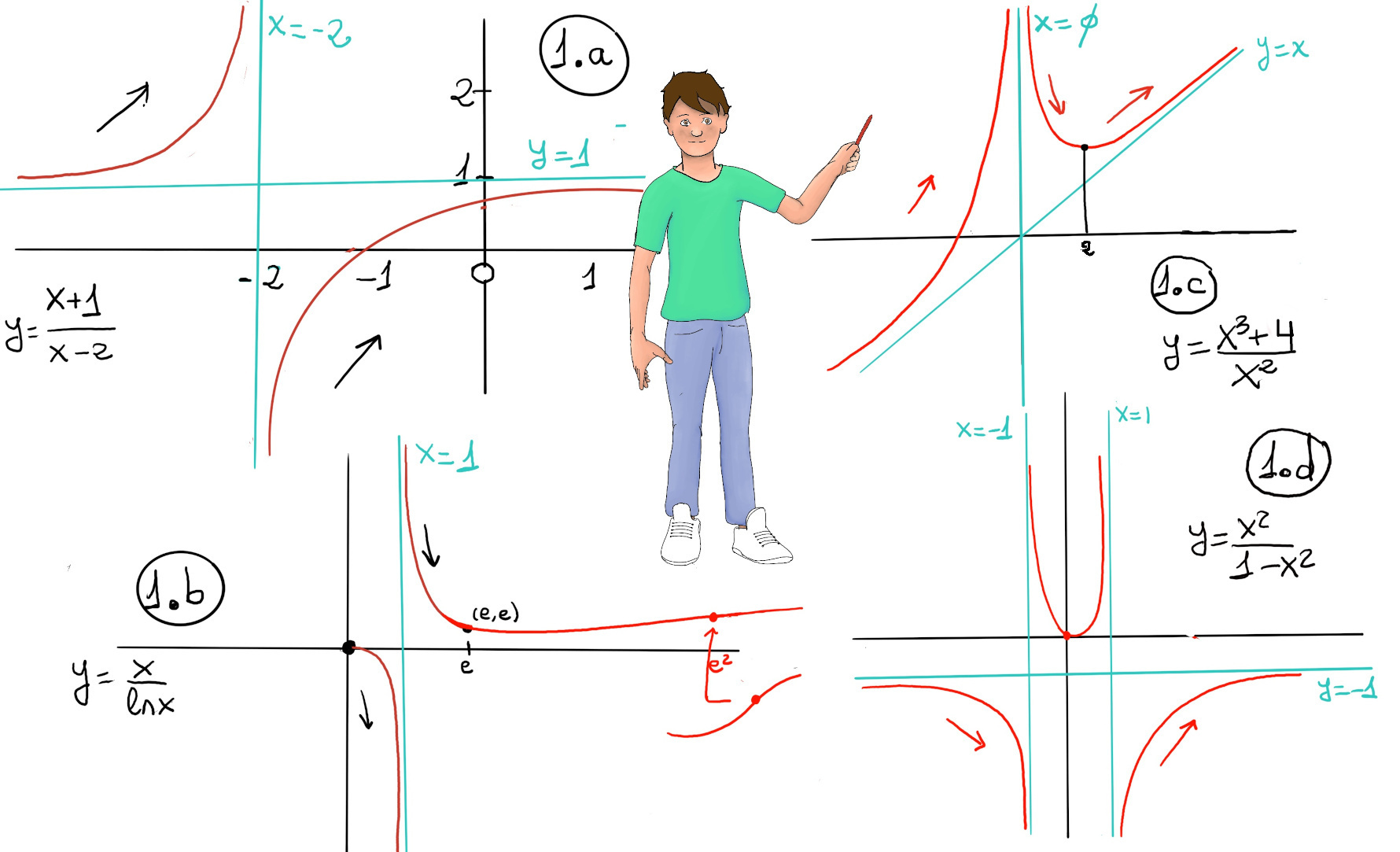
1. Domain = ℝ - {0}. f is not defined at x = 0.

2. $\lim_{x \to 0}\frac{x^{3}+4}{x^{2}} = \frac{4}{0^{+}} = \infty$, x = 0 is a vertical asymptote.

3. $\lim_{x \to \infty}\frac{x^{3}+4}{x^{2}} = \infty, \lim_{x \to -\infty}\frac{x^{3}+4}{x^{2}} = -\infty$.

   When a linear asymptote is not parallel to the x- or y-axis, it is called an oblique asymptote. A function f(x) is asymptotic to y = mx + n (m ≠ 0) if: m = $\lim_{x \to \pm\infty} \frac{f(x)}{x} = m, \lim_{x \to \pm\infty} (f(x) -mx) = n.$

4. m = $\lim_{x \to \pm\infty}\frac{\frac{x^{3}+4}{x^{2}}}{x} = \lim_{x \to \pm\infty}\frac{x^{3}+4}{x^{3}}=1, lim_{x \to \pm\infty} \frac{x^{3}+4}{x^{2}} -x=lim_{x \to \pm\infty} \frac{4}{x^{2}} = 0,$ y =[m = 1, n = 0] x is an oblique asymptote, more details at this link. The plot is shown in Figure 1.c.

Bibliography

1. NPTEL-NOC IITM, Introduction to Galois Theory.
2. Algebra, Second Edition, by Michael Artin.
3. LibreTexts, Calculus. Abstract and Geometric Algebra, Abstract Algebra: Theory and Applications (Judson).
4. Field and Galois Theory, by Patrick Morandi. Springer.
5. Michael Penn, and MathMajor.
6. Contemporary Abstract Algebra, Joseph, A. Gallian.
7. YouTube’s Andrew Misseldine: Calculus. College Algebra and Abstract Algebra.
8. MIT OpenCourseWare 18.01 Single Variable Calculus, Fall 2007 and 18.02 Multivariable Calculus, Fall 2007.
9. Calculus Early Transcendentals: Differential & Multi-Variable Calculus for Social Sciences.