Sketching the Graph of a function

A smile is a curve that sets everything straight, Phyllis Diller.

Recall

Definition. A function f is a rule, relationship, or correspondence that assigns to each element of one set (x ∈ D), called the domain, exactly one element of a second set, called the range (y ∈ E).

The pair (x, y) is denoted as y = f(x). Typically, the sets D and E will be both the set of real numbers, ℝ.

Graphing functions involves the visual representation of a curve that reflects the behavior of a mathematical function on a coordinate plane, also known as the Cartesian plane. It is a two-dimensional space defined by two axes - the x-axis (horizontal) and the y-axis (vertical).

A systematic approach to graphing a function begins by constructing a table containing selected input values and their corresponding output values. By extending this table, we can plot the points on the coordinate plane and observe the pattern they form. Connecting these points reveals the shape of the curve, allowing us to gain insights into the behavior of the function across its domain. This process provides a visual means of understanding the relationships between different variables and aids in interpreting the overall characteristics of the function.

Solved examples

• Linear functions, y = mx + b.

Linear functions are among the easiest to graph, each graph is just a straight line. To plot a linear function, calculate and mark two points on the graph (choose two points that are relatively easy to calculate), and then draw a straight line that passes through both of them. Typically, you can plot the intercepts in the axes and draw a straight line passing through them using a ruler.

Definition. The x-intercept of a graph is the point(s) or x-coordinate of any point on the graph that intersects the x-axis. In other words, it is the value of x when the function (y-coordinate or y-value) is zero.

For example, in a linear function defined by y = mx + b, the x-intercept is the solution to the equation 0 = mx +b , that is, x= −b/m. y = 2x -6, the x-intercept is x = 6/2, that is, (3, 0). y = -2x + 5 (Figure iii), the x-intercept is x = -5/-2 = 5/2, that is, (2.5, 0).

If the equation of a graph is y = -2x + 5, to find the y-intercept, set x = 0 ⇒ y = -2(0) + 5 ⇒ y = 5. Therefore, the y-intercept is (0, 5). In other words, when the equation of a line is written in a slope-intercept form (y = mx + b), the y -intercept can be read immediately from the equation, that is, b, e.g., y = -2x + 5 the y-intercept is (0, 5) (Figure iii).

A linear function is a function of the form y = mx + b, where m is the slope of the line, b is the y-intercept, and −b/m the x-intercept.

• Quadratic functions, y = ax² + bx + c.

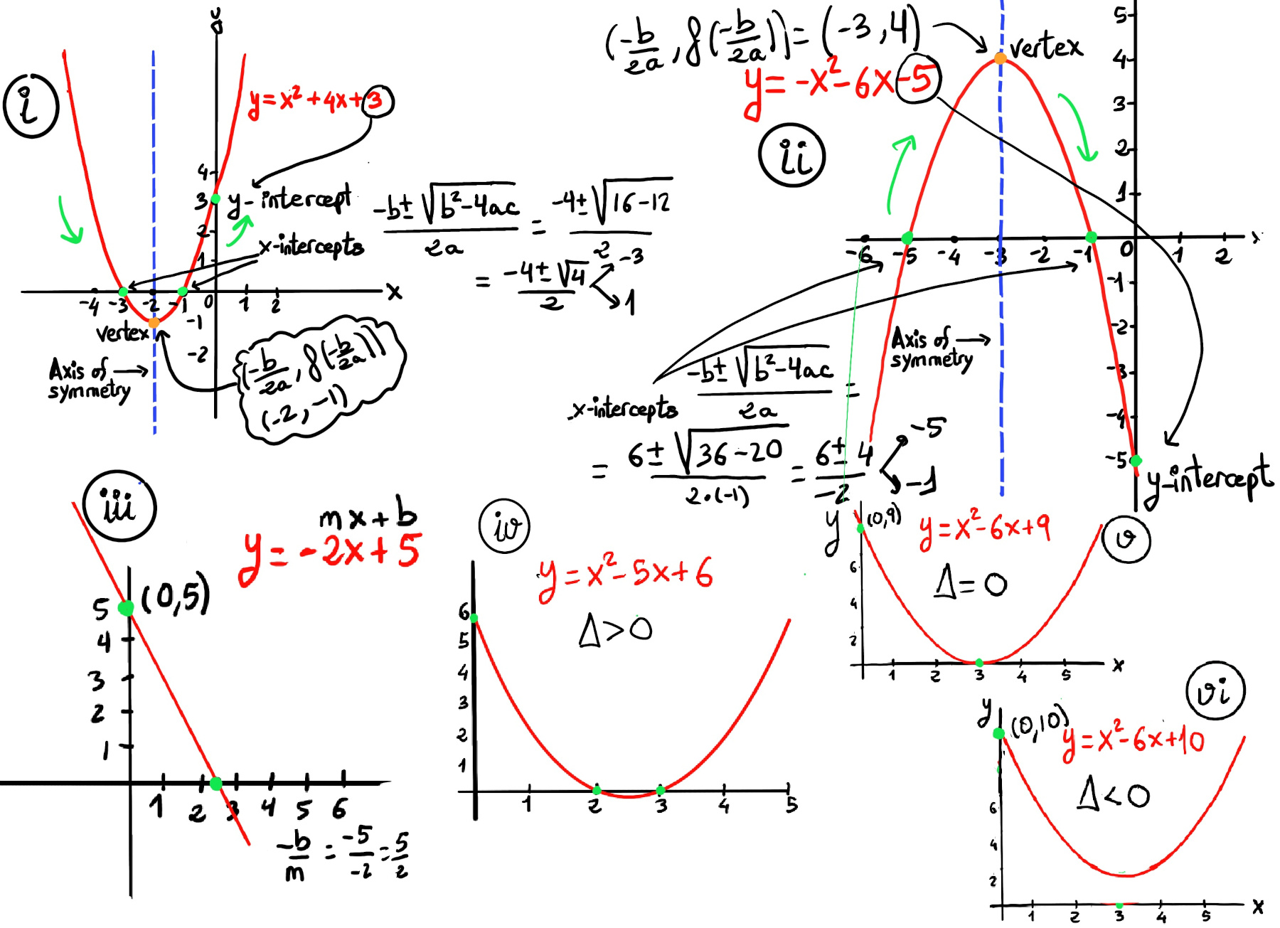
The graph of a quadratic function ax² + bx + c is a parabola. It has an extreme point, called the vertex where the curve changes direction.

If the parabola opens upwards (a > 0), the vertex represents the lowest point on the curve and its y-coordinate is the minimum value of the quadratic function. If the parabola opens downwards (a < 0), the vertex represents the highest point on the curve, and its y-coordinate is the maximum value. In either case, the vertex is a turning point on the graph. The graph is also symmetric with a vertical line drawn through the vertex, called the axis of symmetry $x = \frac{-b}{2a}$, So, the graph of the function is increasing on one side of the axis and decreasing on the other side.

In a quadratic function, we use the quadratic formula, x = $\frac{-b±\sqrt{b^2-4ac}}{2a}$, for the x-intercepts and represent the roots or zeros of the quadratic function. The discriminant can be used to calculate the number of x-intercepts and the type of solutions of the quadratic equation.

1. If the value of the discriminant, b²-4ac, is less than zero, the quadratic equation has two imaginary solutions meaning that the equation does not have any real solution or there are no x-intercepts, e.g., y = $x^2-6x+10, b^2-4ac = 36-40 = -4 < 0,$ (Figure vi).
2. If the value of the discriminant equals zero, then the quadratic equation has a repeated real root meaning the graph of the solution has a single x-intercept, e.g., $x^2-6x+9, b^2-4ac = 36-36 = 0, x = \frac{-b±\sqrt{b^2-4ac}}{2a} = \frac{6±\sqrt{0}}{2} = 3,$ (Figure v)
3. If the value of the discriminant is positive, then the quadratic equation has two real roots meaning the graph of the solution has two distinct intersect, e.g., $x^2-5x+6, b^2-4ac = 25-24 = 0, x = \frac{-b±\sqrt{b^2-4ac}}{2a} = \frac{5±\sqrt{1}}{2}=$ 3 or 2(Figure iv).

• y = $3x-x^{3}$

1. $\lim_{x \to \infty} 3x-x^{3} = -\infty, \lim_{x \to -\infty} 3x-x^{3} = \infty$
2. f’(x) = 3 -3x² = 0 ↭ 3x² = 3 ↭ x² = 1 ↭ x = ±1, f’(x) = (x-1)(x+1), f’’(x) = -6x, hence 0 is an inflection point. f’’(1) = -6 < 0 ⇒ 1 is a local maximum. f’’(-1) = 6 > 0 ⇒ 1 is a local maximum.
3. x < 0, f’’(x) < 0 ⇒ f’ is decreasing ⇒ f is concave downward.
4. x > 0, f’’(x) > 0 ⇒ f’ is increasing ⇒ f is concave upward.
5. Finally, let’s plot our critical points, namely f(1) = 2, f(-1) = -2, f(0) = 0 -Figure 1.e-.

f(-x) =[f(x) = 3x -x³] -3x - (-x)³ = -3x +x³ = - (3x -x³) = -f(x), so f is an even function, it has symmetry about the origin.

• Let’s plot $\frac{x + 1}{x + 2}$

f’(x) = $\frac{1}{(x+2)^2}$ > 0 ∀ x ∈ ℝ, x ≠ -2 ⇒ f is increasing (-∞, -2) and (-2, ∞).

Critical points are those where the derivate is zero or the derivate is not defined, e.g., in our example, x = -2.

$\lim_{x \to -2^{+}}\frac{x+1}{x+2} = \frac{-1}{0⁻} = \infty, \lim_{x \to -2^{-}}\frac{x+1}{x+2} = \frac{-1}{0⁺}= -\infty$

Vertical asymptotes are vertical lines (perpendicular to the x-axis) of the form x = a (where a is a constant) near which the function grows without bound. The line x = a is a vertical asymptote if: $\lim_{x \to a^{-}}f(x)=\pm\infty$ or $\lim_{x \to a^{+}}f(x)=\pm\infty$, e.g., x = -2 is a vertical asymptote of $\frac{x+1}{x+2}$.

$\lim_{x \to \pm\infty}\frac{x+1}{x+2} = 1$

Horizontal asymptotes are horizontal lines (parallel to the x-axis) that the graph of the function approaches as x → ±∞. y = c is a horizontal asymptote if the function f(x) becomes arbitrarily close to c as long as x is sufficiently large or small or more formally: $\lim_{x \to \infty}f(x)=c$ or $\lim_{x \to -\infty}f(x)=c$, e.g., y = 1 is a horizontal asymptote of $\frac{x+1}{x+2}$.

To sum up,

1. f’(x) = ¹⁄_{(x + 2)²} > 0 ∀x ∈ ℝ, x ≠ -2 ⇒ f is increasing (-∞, -2)∪(-2, ∞).
2. $\lim_{x \to -2^{+}}\frac{x+1}{x+2} = \infty, \lim_{x \to -2^{-}}\frac{x+1}{x+2} = -\infty$, x = -2 is a vertical asymptote.
3. $\lim_{x \to \pm\infty}\frac{x+1}{x+2} = 1$, y = 1 is a horizontal asymptote.
4. f’’(x) = ^-2⁄_{(x + 2)³}, x ≠ -2. f’’(x) > 0, x < -2 ⇒ concave upward. f’’(x) < 0, x > -2 ⇒ concave downward.

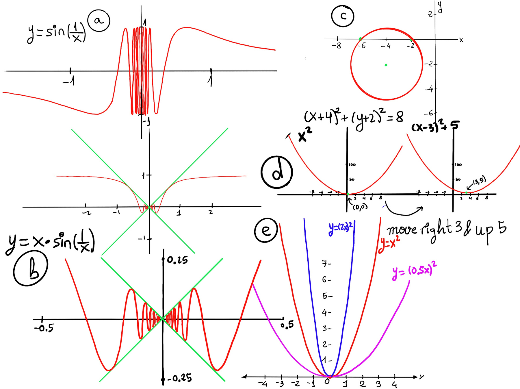
The plot is shown in Figure 1.a.  

• y = $\frac{x^{3}+4}{x^{2}}$

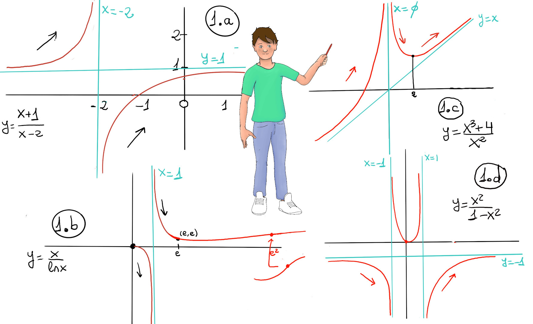
1. Domain = ℝ - {0}. f is not defined at x = 0.

2. $\lim_{x \to 0}\frac{x^{3}+4}{x^{2}} = \frac{4}{0^{+}} = \infty$, x = 0 is a vertical asymptote.

3. $\lim_{x \to \infty}\frac{x^{3}+4}{x^{2}} = \infty, \lim_{x \to -\infty}\frac{x^{3}+4}{x^{2}} = -\infty$.

   When a linear asymptote is not parallel to the x- or y-axis, it is called an oblique asymptote. A function f(x) is asymptotic to y = mx + n (m ≠ 0) if: m = $\lim_{x \to \pm\infty} \frac{f(x)}{x} = m, \lim_{x \to \pm\infty} (f(x) -mx) = n.$

4. m = $\lim_{x \to \pm\infty}\frac{\frac{x^{3}+4}{x^{2}}}{x} = \lim_{x \to \pm\infty}\frac{x^{3}+4}{x^{3}}=1, lim_{x \to \pm\infty} \frac{x^{3}+4}{x^{2}} -x=lim_{x \to \pm\infty} \frac{4}{x^{2}} = 0,$ y =[m = 1, n = 0] x is an oblique asymptote.

5. f’(x) = $\frac{3x^{4}-(x^{3}+4)2x}{x^{4}}= \frac{3x^{4}-2x^{4}-8x}{x^{4}}= \frac{x^{3}-8}{x^{3}}$, f’(x) = 0 ⇒ x = 2. Futhermore, x < 0, f’(x) > 0 ⇒ f increasing ↗. 0 < x < 2, f’(x) < 0 ⇒ f decreasing ↘. x > 2, f’(x) > 0 ⇒ f increasing ↗. The plot is shown in Figure 1.c.

Bibliography

1. NPTEL-NOC IITM, Introduction to Galois Theory.
2. Algebra, Second Edition, by Michael Artin.
3. LibreTexts, Calculus.
4. Field and Galois Theory, by Patrick Morandi. Springer.
5. Michael Penn, and MathMajor.
6. Contemporary Abstract Algebra, Joseph, A. Gallian.
7. YouTube’s Andrew Misseldine: Calculus, College Algebra and Abstract Algebra.
8. Calculus Early Transcendentals: Differential & Multi-Variable Calculus for Social Sciences.
9. blackpenredpen.