Numerical integration.

The more I learn about people, the more I like dogs and I don’t even have a dog, Apocalypse, Anawim, #justtothepoint.

Recall

Antiderivatives are fundamental concepts in calculus. They are the inverse operation of derivatives.

Given a function f(x), an antiderivative, also known as indefinite integral, F, is the function that can be differentiated to obtain the original function, that is, F’ = f, e.g., 3x² -1 is the antiderivative of x³ -x +7 because $\frac{d}{dx} (x^3-x+7) = 3x^2 -1$. Symbolically, we write F(x) = $\int f(x)dx$.

The process of finding antiderivatives is called integration.

The Fundamental Theorem of Calculus states roughly that the integral of a function f over an interval is equal to the change of any antiderivate F (F'(x) = f(x)) between the ends of the interval, i.e., $\int_{a}^{b} f(x)dx = F(b)-F(a)=F(x) \bigg|_{a}^{b}$

Numerical integration

In analysis, numerical integration comprises a broad family of algorithms for calculating the numerical value of a definite integral when analytical solutions are challenging.

All numerical approximations of the integral $\int_{a}^{b} f(x)dx$ will start with a partition of the interval [a, b] into n equal parts, a = x₀ < x₁ < ··· < x_n = b, Δx = x_i-x_i-1, y₀ = f(x₀), y₁ = f(x₁), ···, y_n = f(x_n).

We define the left Riemann sum as follows = (y₀ + y₁ + ··· + y_n-1)Δx = f(x₀)Δx + f(x₁)Δx + ··· + f(x_n-1)Δx = $\sum_{k=0}^{n-1} f(x_k)Δx$ where the chosen point of each subinterval (x_i-1, x_i) of the partition is the left-hand point x_i-1. The right Riemann sum is defined similarly = (y₁ + y₂ + ··· + y_n)Δx = f(x₁)Δx + f(x₂)Δx + ··· + f(x_n)Δx = $\sum_{k=1}^{n} f(x_k)Δx$ -Figure 1.b.- where the chosen point of each subinterval (x_i-1, x_i) of the partition is the right-hand point x_i.

If the function is continuous and monotonically decreasing/increasing, then the left Riemann sum overestimates/underestimates the integral and the right Riemann sum underestimates/overestimates it.

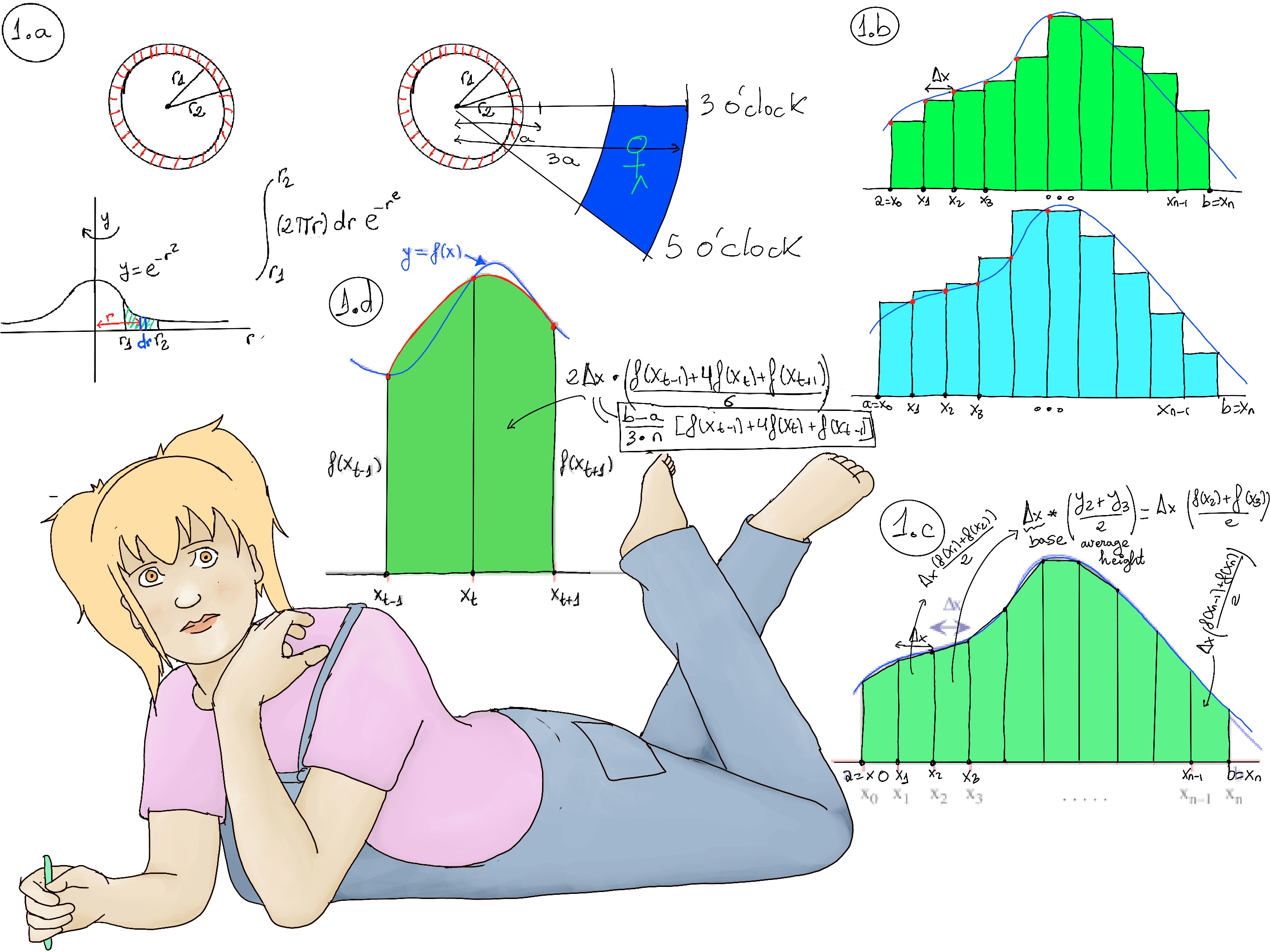
A trapezoid is a four-sided region with two opposite sides parallel. Given a partition of [a, b] as above, we can define the associated trapezoid sum to correspond to the area shown below (Figure 1.c.). The area of a trapezoid is the average length of the parallel sides times the distance between them, e.g., base * average_height = Δx(^y₂+y₃⁄₂). Adding all the areas of the individual trapezoids together, gives the trapezoid sum: $Δx(\frac{y_0+y_1}{2} + \frac{y_1+y_2}{2} + ··· + \frac{y_{n-1}+y_n}{2}) = Δx(\frac{y_0}{2} + y_1 + y_2 + ··· y_{n-1}+\frac{y_n}{2})$ = $\frac{left Riemann Sum + Right Riemann Sum}{2}$ -Figure 1.c.-. The trapezoid sum is the average of the left- and right-hand Riemann sums.

Simpson’s rule gives us another approximation of the integral. Again, we start by partitioning [a, b] into intervals all of the same width, but this time we must use an even number of intervals, so n needs to be even. We are going to use a parabola through the three points (x_k-1, f(x_k-1)), (x_k, f(x_k)), and (x_k+1, f(x_k+1)), and the area under the parabola (Figure 1.d., it is left as an exercise) equals base*average height = $2Δx(\frac{y_{k-1}+4y_k+y_{k+1}}{6})=\frac{b-a}{3n}[f(x_{k-1})+4f(x_k)+f(x_{k+1})]$, and the total sum is $\frac{Δx}{3}((y_0+4y_1+y_2) + (y_2+4y_3+y_4) + ··· (y_{n-2}+4y_{n-1}+y_n))$ = 🚀

=[🚀] $\frac{Δx}{3}(y_0 +4y_1 +2y_2 +4y_3 + ··· + 2y_{n-2}+4y_{n-1}+y_n)$ -Figure 1.d.- Here, the coefficients 1, 4, and 2 alternate. Simpson's Rule is more accurate than the trapezoidal rule for approximating integrals because it uses a quadratic interpolation to model the curve. It provides a good balance between simplicity and accuracy for numerical integration. Futhermore, it is exact when integrating polynomials of degree 3 or less.

Examples

• $\int_{1}^{2} \frac{dx}{x}= ln(x)\bigg|_{1}^{2} = ln(2) -ln(1) = ln(2) $ ≈ 0.693147 where b = x₂ = 2, y₂ = ¹⁄₂, x₁ = 3/2, y₁ = 2/3, a = x₀ = 1, y₀ = 1, b -a = 1, n = 2, $\Delta x = \frac{b-a}{n} = \frac{1}{2},$ Figure 1.a.

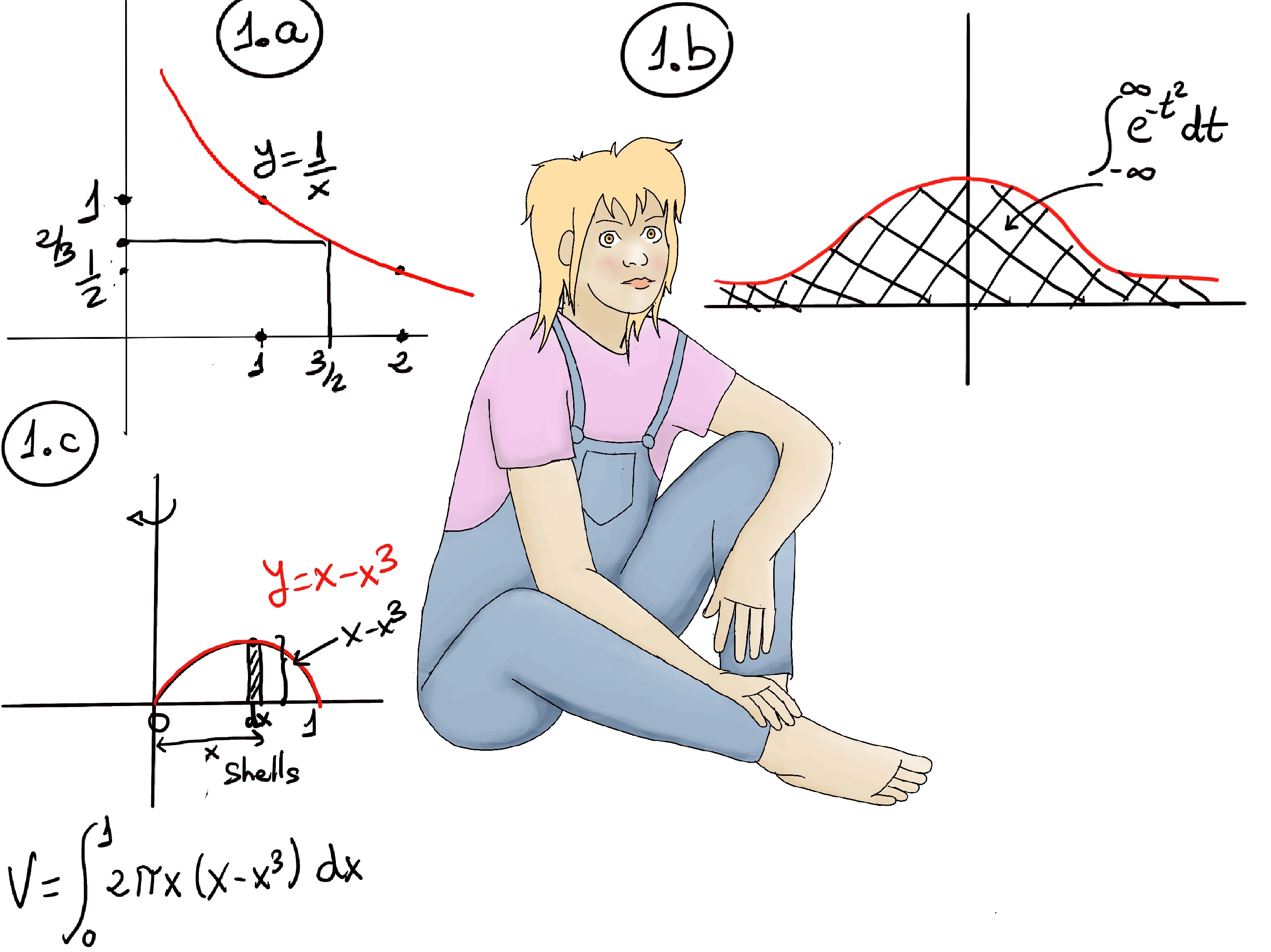
1. Trapezoidal rule. $\Delta x(\frac{1}{2}y_0 + y_1 + \frac{1}{2}y_2)=\frac{1}{2}(\frac{1}{2}·1 + \frac{2}{3} + \frac{1}{2}·\frac{1}{2}) = \frac{1}{2}(\frac{6}{12}+\frac{8}{12}+\frac{3}{12}) = \frac{1}{2}·\frac{17}{12} = \frac{17}{24}$ ≈ 0.7083 it is obviously not a very good approximation 😞, but it was expected we should split the interval into more subintervals.

2. Sympson’s rule. $\frac{\Delta x}{3}(y_0 +4y_1 +y_2) = \frac{1}{6}(1 + 4·\frac{2}{3}+\frac{1}{2}) ≈ 0.69444$ that is surprisingly a relatively good approximation of the correct value.

• Approximate $\int_{0}^{1} \sqrt{1-x^2}dx$. We know that $\int_{0}^{1} \sqrt{1-x^2}dx = \frac{π}{4} ≈ 0.7853981635$

Now, we need to compute the function values at the endpoints of the subintervals. For n = 4, the endpoints are: $x_0 = 0, x_1 = \frac{1}{4}, x_2 = \frac{1}{2}, x_3 = \frac{3}{4}, x_4 = 1, f(x_0)=\sqrt{1−0^2} =1, f(x_1) = \sqrt{1 - \left(\frac{1}{4}\right)^2} = \sqrt{\frac{15}{16}}, f(x_2) = \sqrt{1 - \left(\frac{1}{2}\right)^2} = \sqrt{\frac{4}{4}-\frac{1}{4}} = \sqrt{\frac{3}{4}}, f(x_3) = \sqrt{1 - \left(\frac{3}{4}\right)^2} = \sqrt{\frac{16}{16}-\frac{9}{16}} = \sqrt{\frac{7}{16}}, f(x_4) = \sqrt{1 - 1^2} = 0$

1. Trapezoidal rule. $\Delta x(\frac{1}{2}y_0 + y_1 + y_2 + y_3 + \frac{1}{2}y_4)=\frac{1}{4}(\frac{1}{2} + \sqrt{\frac{15}{16}} + \sqrt{\frac{3}{4}} + \sqrt{\frac{7}{16}} + 0) ≈ 0.748927$

2. Sympson’s rule. $\frac{\Delta x}{3}(y_0 +4y_1 + 2y_2 + 4y_3 + y_3) = \frac{1}{12}(1 + 4·\sqrt{\frac{15}{16}} + 2·\sqrt{\frac{3}{4}} + 4·\sqrt{\frac{7}{16}} + 0) ≈ 0.77089878 $

Bibliography

1. NPTEL-NOC IITM, Introduction to Galois Theory.
2. Algebra, Second Edition, by Michael Artin.
3. LibreTexts, Calculus. Abstract and Geometric Algebra, Abstract Algebra: Theory and Applications (Judson).
4. Field and Galois Theory, by Patrick Morandi. Springer.
5. Michael Penn, and MathMajor.
6. Contemporary Abstract Algebra, Joseph, A. Gallian.
7. YouTube’s Andrew Misseldine: Calculus. College Algebra and Abstract Algebra.
8. MIT OpenCourseWare 18.01 Single Variable Calculus, Fall 2007 and 18.02 Multivariable Calculus, Fall 2007.
9. Calculus Early Transcendentals: Differential & Multi-Variable Calculus for Social Sciences.