Linear and Quadratic Approximation

An old joke that Adam told to Even, but makes cents, Once a man said to God “What’s a million years to you?”, and God said “A second.” So the man said to God “What’s a million dollars to you?”, and God said “A penny.” So the man said to God “Would you give me a penny?” And God replied, “Sure, just wait a second.”

Recall

Definition. A function f is a rule, relationship, or correspondence that assigns to each element of one set (x ∈ D), called the domain, exactly one element of a second set, called the range (y ∈ E).

The pair (x, y) is denoted as y = f(x). Typically, the sets D and E will be both the set of real numbers, ℝ.

Linear and quadratic approximations are methods used to approximate a complicated function with simpler, linear or quadratic functions near a specific point. This is useful when the exact value of the function at that point is difficult to calculate, computationally costly, or tedious to find. These approximations are valuable in calculus and numerical analysis for estimating the behavior of functions near certain points or for simplifying calculations.

Linear approximation

Linear approximation does a very good job of approximating values of f(x) as long as we stay near x = a, that is, in the neighborhood around a. If a function y = f(x) is differentiable at a point (a, f(a)), the function looks like its tangent line in a small open interval containing a. It allows us to approximate the original function f (it is sometimes computationally too costly -in terms of resources- or algebraically complicated) with a simpler function L that is linear.

The tangent line is f(x) = f(x₀) + f’(x₀)(x-x₀) and touches the curves at this particular point (x₀, y₀)

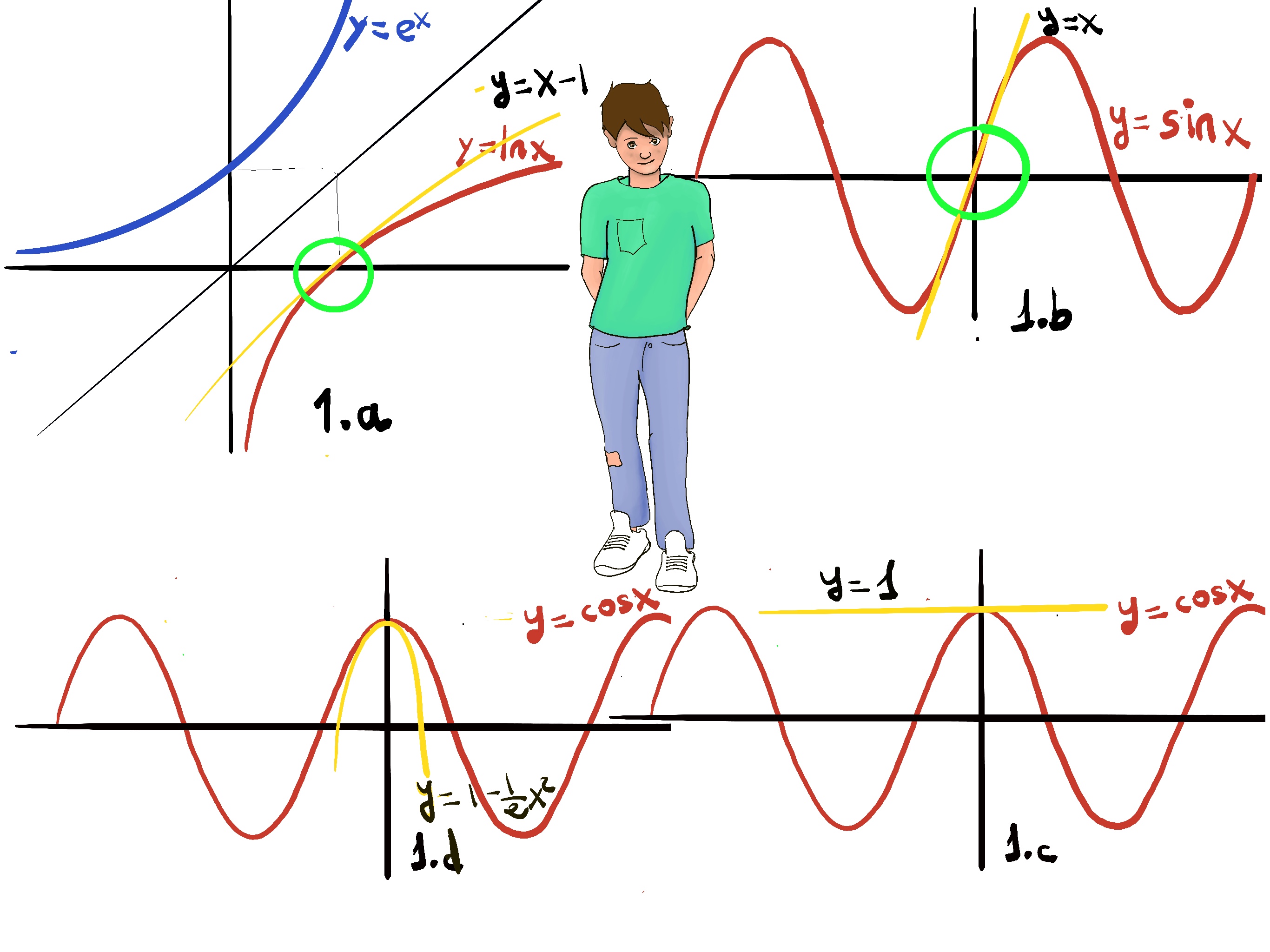
Let x₀=1, e.g., $x_0=1, ln(1) = 0, ln’(x)=\frac{1}{x}, ln’(1)=\frac{1}{1} = 1$⇒ lnx ≅ x - 1 (-Figure 1.a.-)

How to Perform Linear Approximation

1. Find the point (x₀ ,f(x₀)) on the curve where you want to approximate the function.
2. Calculate the derivative f’(x₀) to find the slope of the tangent line at that point.
3. Use the point-slope form to write the equation of the tangent line, f(x) = f(x₀) + f’(x₀)(x-x₀) where (x₀, f(x₀)) is a point on the tangent line, and f’(x₀) is the slope.
4. Use this linear equation to evaluate and estimate the value of the function at points close to x₀.

Let x₀=0, f(x) = f(0) + f’(0)(x). Other examples are:

1. sinx ≅ x (1.b), e.g., sin(0.1) = 0.0998334166 ≈ 0.1.
2. cosx ≅ 1 (1.c). e.g., cos(0.1) = 0.9950041653 ≈ 1.
3. e^x ≅ 1+x, e.g. e^0.2 = 1.2214027582 ≅ 1+0.2 = 1.2.
4. ln(1+x) ≅ x, e.g. ln(1+0.1) ≅ 0.0953101798, which is close to 0.10.
5. (1+x)^r ≅ 1 +rx

   (1+x)^r, f(x) ≅ f(0) + f’(0)(x) = 1 +r(1+x)^r-1|_x=0·x = 1 + rx,, e.g., x = 0, r = 3, (1+0.1)³ = 1.331 ≅ 1 +3·(0.1) = 1.3. The approximation yields 13, which is close to the actual value of 1.331.

   

• Approximate the number $\sqrt[4]{1.1}$

So let f(x) = $\sqrt[4]{x}$. Obviously, 1 is relatively close to 1.1 and we take x₀ = 1. Then, the tangent line is y = f(x₀) + f’(x₀)(x -x₀) =[f’(x)=$\frac{1}{4x^{\frac{3}{4}}}, f’(1)=\frac{1}{4·1^{\frac{3}{4}}}=\frac{1}{4}$]

$\sqrt[4]{1.1} = 1.024114… ≈ \sqrt[4]{1}+\frac{1}{4}(1.1 -1) = 1+\frac{1}{4}·0.1 = 1.025.$

• Find linear approximation near x = 0 of $\frac{e^{-3x}}{\sqrt{1+x}}$

$\frac{e^{-3x}}{\sqrt{1+x}} = e^{-3x}(1+x)^{-1/2} ≅ (1-3x)(1-\frac{1}{2}x) ≅~ 1 -3x -\frac{1}{2}x +\frac{3}{2}x^{2} ≅ 1 -3x -\frac{1}{2}x ≅ 1 -\frac{7}{2}x$. Observe that we do not care about quadratic and higher other terms and consider them as negligible as long as we are close enough to 0.

Besides, $e^x = 1 +x ⇒ e^{-3x} ≅ 1 +f’(0)x = 1 + (-3x)$. Similarly, (1+x)^-1/2 ≅ 1 + f’(0)x, and f’(0) = -1/2(1+x)^-3/2|_x=0 = -1/2, hence (1+x)^-1/2 ≅ 1 + ^-1⁄₂x

The challenging limit $\lim_{x \to 0} \frac{sin(x)}{x}$ is an indeterminate form (0/0). It is easy to show that the linearization of f(x) = sin(x) at the point (0, 0) is given by x, hence for values x near 0, sin(x)≈ x, and therefore $\frac{sin(x)}{x}≈\frac{x}{x} = 1$ which makes reasonable the fact that $\lim_{x \to 0} \frac{sin(x)}{x}$ =1.

Quadratic approximation

When using approximation you sacrifice some accuracy for the ability to perform complex calculations easily and fast. Quadratic approximation is used when the linear approximation is not good or close enough. The basic formula for quadratic approximation with x₀ is:

f(x) ≅ f(x₀) + f’(x₀)(x-x₀) + ^{f’’(x₀)}⁄₂(x-x₀)², and this is generally enough for x ≅ x₀.

It gives a best-fit parabola to a function. Ideally, the quadratic approximation of a quadratic function, say f(x) = a +bx +cx² should be identical to the original function.

f(x) = a +bx +cx²
f’(x) = b + 2cx
f’’(x) = 2c

Set the base x₀ as zero. Next, we try to recover the values of a, b, and c. f(0) = a
f’(0) = b
f’’(0) = 2c ⇒ c = ^f’’(0)⁄₂

f(x) ≅ f(x₀) + f’(x₀)(x-x₀) + ^{f’’(x₀)}⁄₂(x-x₀)² where x ≅ x₀, say x = 0, hence f(x) ≅ f(0) + f’(0)(x) + ^f’’(0)⁄₂x² where x ≅ 0, f(x) ≅ a +bx + ^2c⁄₂x² = a +bx +cx²

How to Perform Quadratic Approximation

1. Find the point (x₀ ,f(x₀)) on the curve where you want to approximate the function.
2. Calculate the first f’(x₀) and second derivatives f’(x₀) at that point.
3. Plug these values into the quadratic approximation formula to get the quadratic polynomial that approximates the function near x₀, f(x) = f(x₀) + f’(x₀)(x-x₀) + ^{f’’(x₀)}⁄₂(x-x₀)².
4. Use this quadratic polynomial to evaluate and estimate the value of the function at points close to x₀.

• ln(1+x) ≅ x -^x2⁄₂ (if x ≅ 0).
• sinx ≅ x (if x ≅ 0).
• cosx ≅ 1 -¹⁄₂x² (1.d., if x ≅ 0).
• e^x ≅ 1 + x + ¹⁄₂x² (if x ≅ 0).
• (1+x)^r = 1 +rx + ^r(r-1)⁄₂x² (if x ≅ 0).

The linear approximation of cosx near 0 is the straight horizontal line y = 1. This doesn’t seem like a very good approximation. The quadratic approximation to the graph of cos(x) is a parabola that opens downward, cosx ≅ 1 -¹⁄₂x² (1.d.), this is much closer to the shape of its graph than the line y = 1.

• Find quadratic approximations for f(x) = ln(1.1).

f(x) ≈ $f(x_0)+f’(x_0)(x-x_0)+\frac{f’’(x_0)}{2}(x-x_0)^2$.

Let f(x) = ln(x), x₀ = 1, f’(x) = $\frac{1}{x}, f’’(x) = \frac{-1}{x^2}$.

ln(1.1) = $ln(1+\frac{1}{10}) ≈ ln(1)+\frac{1}{1}(1+\frac{1}{10}-1)+\frac{-1}{2·1^2}(1+\frac{1}{10}-1)^2 = \frac{1}{10}-\frac{1}{2}\frac{1}{100}=0.095$

• Find the linear and quadratic approximations for f(x) = $\sqrt x$ near x = 4.

f’(x) = $\frac{1}{2\sqrt{x}} = \frac{1}{2}·x^{\frac{-1}{2}} =$ , f’’(x)= $\frac{1}{2}·\frac{-1}{2}·x^{\frac{-1}{2}-1} = \frac{-1}{4·x^{\frac{3}{2}}} = \frac{-1}{4·x·\sqrt{x}}$, then

1. Linear approximation, L(x) = f(4) + f’(4)(x-4) = $2 + \frac{1}{4}(x-4) = 1 + \frac{1}{4}x$.
2. Quadratic approximation, Q(x) = f(x) + f’(4)(x-4) + ¹⁄₂f’’(4)·(x -4)² = $1 + \frac{1}{4}x -\frac{1}{2}·\frac{-1}{4·4·2}(x-4)^2 = 1 + \frac{1}{4}x -\frac{1}{64}(x-4)^2 = 1 + \frac{1}{4}x -\frac{1}{64}·x^2-\frac{16}{64}+\frac{8}{64}x = \frac{3}{4} + \frac{3}{8}x -\frac{1}{64}·x^2.$

• Find quadratic approximations for f(x)=xe^-2x near x=1 and g(x)=e^-3x(1+x)^-1/2 near x=0.

f(1)=e^-2
f’(x)=e^-2x-2xe^-2x=e^-2x(1-2x) ⇒ f’(1)= -e^-2
f’’(x)=-2e^-2x-2e^-2x(1-2x)=-2e^-2x(2-2x)=-4e^-2x(1-x) ⇒ f’’(1)=0.

f(x) ≅ e^-2 -e^-2(x-1)

$e^{-3x}(1+x)^\frac{-1}{2} ≅ (1 -3x + \frac{9x^{2}}{2})(1 +\frac{-1}{2}x + \frac{3}{8}x^{2}) ≅ 1 -3x + \frac{9x^{2}}{2} +\frac{-1}{2}x + \frac{3}{2}x^{2} + \frac{3}{8}x^{2} ≅ 1 +\frac{-7}{2}x + \frac{51}{8}x^{2} $ 💡O(x³) ≅ 0.

Bibliography

1. NPTEL-NOC IITM, Introduction to Galois Theory.
2. Algebra, Second Edition, by Michael Artin.
3. LibreTexts, Calculus.
4. Field and Galois Theory, by Patrick Morandi. Springer.
5. Michael Penn, and MathMajor.
6. Contemporary Abstract Algebra, Joseph, A. Gallian.
7. YouTube’s Andrew Misseldine: Calculus, College Algebra and Abstract Algebra.
8. Calculus Early Transcendentals: Differential & Multi-Variable Calculus for Social Sciences.
9. blackpenredpen.