Derivate

If you wish to make an apple pie from scratch, you must first invent the universe, Carl Sagan

Definition. Let y = f(x) be a function. The tangent line is the straight line that just touches the curve of the given function at one particular point, say P = (x₀, y₀) -1.a.-, matching the curve's slope there.

The tangent line’s equation at a given point P = (x₀, y₀) is y - y₀ = m (x - x₀), where y₀ = f(x₀). The slope m of a tangent line at a point P(x₀, y₀) is its derivative at that very point, m = f’(x₀). In other words, the derivative of a function at a given point f’(x₀) is the slope of the tangent line at that point. 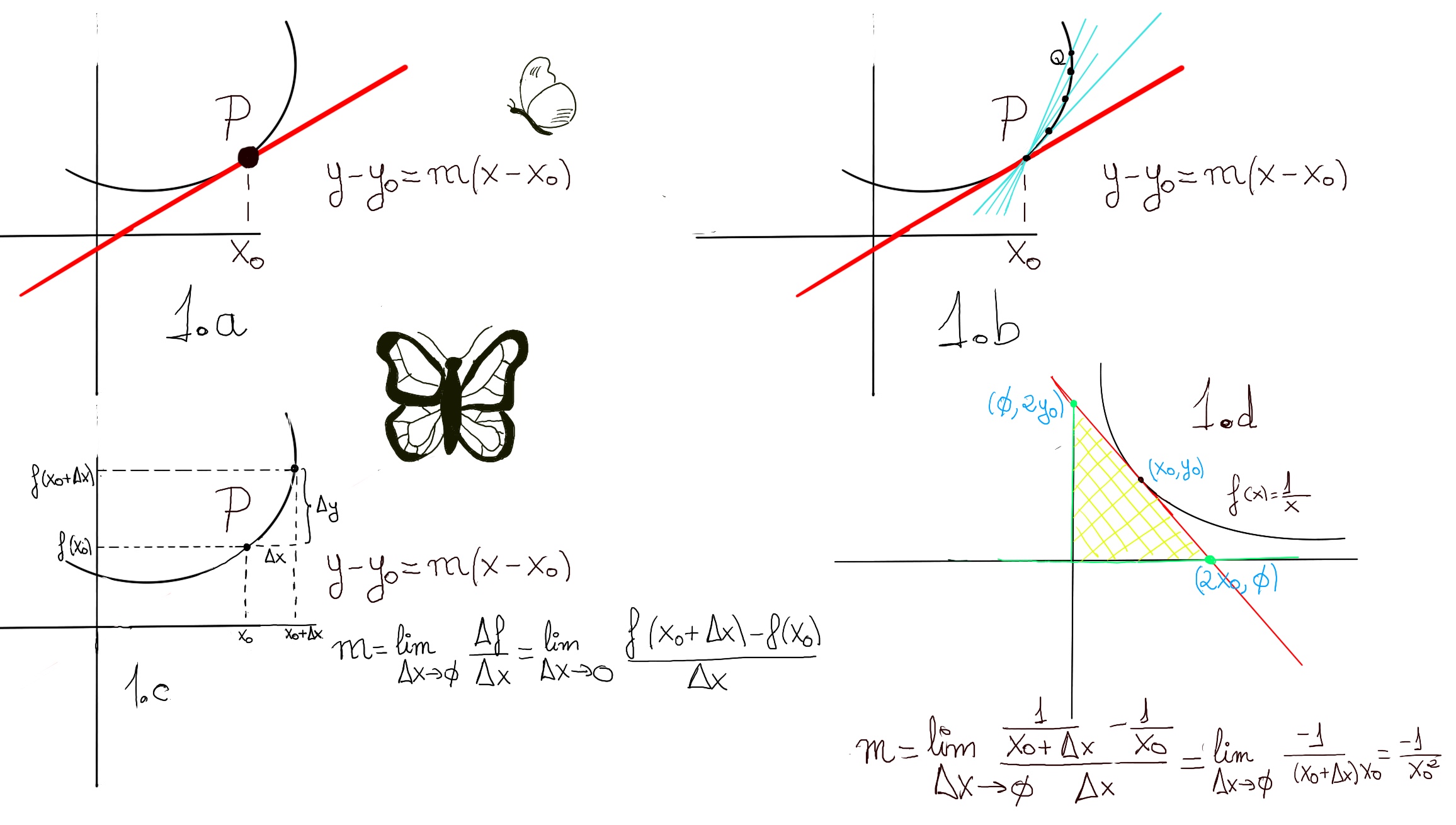  The slope of the tangent line is the limit of the slopes of the secant lines PQ as they approach the tangent line or as Q approach P (P is obviously fixed), that is -1.b., 1.c.-,

m = f’(x₀) = $\lim_{\Delta x \to 0} \frac{\Delta f}{\Delta x}$ = $\lim_{\Delta x \to 0} \frac{f(x_0+\Delta x) -f(x_0)}{\Delta x}$

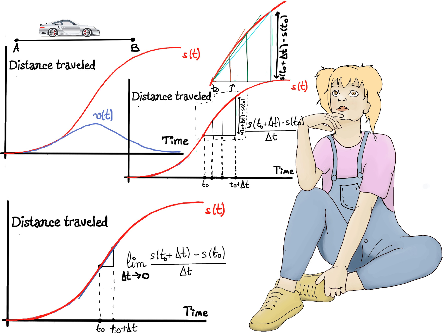
Let’s imagine a car 🚗 that starts at some city A (Madrid), speeds up, and then slows down to a stop at some city B (Barcelona). We could graph this motion (s(t)), letting the vertical axis (y) represents the distance traveled by the vehicle (measured in units such as meters, kilometers, miles, etc.), and the horizontal axis (x) represents the time taken to travel the distance (measured in units such as seconds, minutes, hours, etc.).

Initially the curve is quite shallow (commercial cars are typically slow to start), then for the next seconds, as the car speeds up, the distance traveled in a given time get larger or, in other words, the curve become steeper, and as the car slows towards the end, the curve shallows out again. We can also plot velocity.

The average speed during an entire motion can be thought of as the average of all speedometer readings and is often calculated using the following formula $\frac{distance~ traveled}{time~ of~ travel}$; more formally, $\frac{s(t_0 + \Delta t)-s(t_0)}{\Delta t}$.

Velocity is the rate of change of an object displacement or position with respect to time. Instantaneous velocity is the velocity of an object in motion at a specific point in time. It is the limit of the average velocity when the time interval approaches zero and is the slope of the tangent line at that particular point on the graph (distance traveled or position versus time), $\lim_{\Delta t \to 0} \frac{s(t_0 + \Delta t)-s(t_0)}{\Delta t}$ (Figure below).  

• Example: f(x)=¹⁄_x. 1.d.

  $\frac{f(x_0+\Delta x) -f(x_0)}{\Delta x} = \frac{\frac{1}{x_0+\Delta x} -\frac{1}{x_0}}{\Delta x} = \frac{1}{\Delta x} \frac{x_0-x_0-\Delta x}{(x_0+\Delta x)x_0} = \frac{1}{\Delta x} \frac{-\Delta x}{(x_0+\Delta x)x_0} = \frac{-1}{(x_0+\Delta x)x_0}$

And therefore, $\lim_{\Delta x \to 0} \frac{f(x_0+\Delta x) -f(x_0)}{\Delta x} = \lim_{\Delta x \to 0}\frac{-1}{(x_0+\Delta x)x_0} = \frac{-1}{x_0^{2}}$

Observe that the slope is negative and as x₀ → ∞, the line tangent has less and less slope.

Let’s calculate or compute the areas of triangles enclosed by the axes and the tangent line to y = ¹⁄_x.

The tangent line equation is y - y₀ = f’(x₀)(x - x₀) ↭ y - y₀ = ^-1⁄_x0² (x - x₀).

The x-intercept is the point where the tangent line crosses the x-axis, that is, y = 0.

y - y₀ = 0 - y₀ = 0 - ¹⁄_x0 = ^-1⁄_x0² (x - x₀) = ^-x⁄_x0²+¹⁄_x0 ⇨

$\frac{x}{x_0^{2}}=\frac{2}{x_0}$ ⇨ x = 2x₀. The x-intercept is (2x₀, 0).

The y-intercept is the point where the tangent line crosses the y-axis, that is, x = 0. Because of symmetry (y = ¹⁄_x ↔ xy = 1 ↔ x = ¹⁄_y), the y-intercept is (0, 2y₀).

Finally, the area of a triangle is defined as the region enclosed by it three sides. It is equal to half of the base times height, i.e., A = ¹⁄₂bh=¹⁄₂(2x₀)(2y₀) =[y₀ = ¹⁄_x0] 2.

For convenience’s sake, we normally do not use x₀, just x, and consider that x is fixed, but $\Delta x$ moves towards zero. Another widely used definition of derivate is f'(x) = $\lim_{h \to 0} \frac{f(x+h) -f(x)}{h}.$

Differential

The term differential is used in calculus to refer to an infinitesimal, that is, an infinitely small difference or change in some varying quantity or variable. It is possible to relate to infinite small changes of various variables to each other using derivatives.

For example, if x is a variable, then a small change in the value of x is often denoted $\Delta x$. The differential dx represents an infinitely small change in the variable x.

Historically, the derivative was thought of as a ratio of infinitesimals: $\frac{dy}{dx}$, where dy is an infinitesimal change in y and dx is an infinitesimal change in x. This interpretation is based on the idea that if dx is an infinitesimally small change in x, then the corresponding change in y, denoted as dy, can be approximated by the derivative times dx. If y is a function of x, then the differential dy of y is related to dx by dy ≈ f'(x)dx or equivalently $\frac{dy}{dx} = f’(x)$.

Conclusion

The derivative of a function at a chosen input value, when it exists, is the slope of the tangent line to the graph of the function at that point. It is the instantaneous rate of change, the ratio of the instantaneous change in the dependent variable to that of the independent variable.

Definition. A function f(x) is differentiable at a point “a” of its domain, if its domain contains an open interval containing “a”, and the limit $\lim _{h \to 0}{\frac {f(a+h)-f(a)}{h}}$ exists, f’(a) = L = $\lim _{h \to 0}{\frac {f(a+h)-f(a)}{h}}$. More formally, for every positive real number ε, there exists a positive real number δ, such that for every h satisfying 0 < |h| < δ, then |L-$\frac {f(a+h)-f(a)}{h}$|< ε.

Examples

• Let’s calculate f’(x) where f(x) = $\sqrt{x}$

$f’(x) = \lim_{\Delta x \to 0} \frac{f(x+\Delta x) -f(x)}{\Delta x} = \lim_{\Delta x \to 0} \frac{\sqrt{x+\Delta x} -\sqrt{x}}{\Delta x} = \lim_{\Delta x \to 0} \frac{\sqrt{x+\Delta x} -\sqrt{x}}{\Delta x} \frac{\sqrt{x+\Delta x} +\sqrt{x}}{\sqrt{x+\Delta x} +\sqrt{x}} = \lim_{\Delta x \to 0} \frac{x+\Delta x-x}{\Delta x(\sqrt{x+\Delta x} +\sqrt{x})} = \lim_{\Delta x \to 0} \frac{\Delta x}{\Delta x(\sqrt{x+\Delta x} +\sqrt{x})} = \lim_{\Delta x \to 0} \frac{1}{\sqrt{x+\Delta x} +\sqrt{x}} = \frac{1}{2\sqrt{x}}$

• Compute f’(0) where f(x) = |x|

$f’(0) = \lim_{\Delta x \to 0} \frac{f(0+\Delta x) -f(0)}{\Delta x} = \lim_{\Delta x \to 0} \frac{|0+\Delta x| -|0|}{\Delta x} = \lim_{\Delta x \to 0} \frac{|\Delta x|}{\Delta x}$

$\lim_{\Delta x \to 0⁺} \frac{|\Delta x|}{\Delta x} = \lim_{\Delta x \to 0⁺} \frac{\Delta x}{\Delta x} = 1. \lim_{\Delta x \to 0⁻} \frac{|\Delta x|}{\Delta x} = \lim_{\Delta x \to 0⁻} \frac{-\Delta x}{\Delta x} = -1,$ the two one-sided limits are different, and so f’(0) does not exist.

• Find the equation of the tangent line to the function y = f(x) = x³ +4x -6 at the point x = 2.

f(2) = 2³ +4·2 -6 = 8 +8 -6 = 10. This gives the point (2, 10).

$\lim_{h \to 0} \frac{f(2+h)-f(2)}{h} = \lim_{h \to 0} \frac{(2+h)^3+4(2+h)-6-(2^3+4·2-6)}{h}$ [(a+b)³ = a³ +3a²b +3ab² +b²] $\lim_{h \to 0} \frac{h^3+2^3+3·4·h+3·2·h^2+8+4h-6-10}{h} = \lim_{h \to 0} \frac{h^3+6h^2+16h}{h} = \lim_{h \to 0} h^2+6h+16 = 16$ ⇒ The slope of the tangent line at 2 is f’(2) = 16.

Recall that the point-slope form of the equation of a line is given by: y - y₀ = m(x - x₀) where (x₀, y₀) is a point on the line and m (f’(x₀)) is the slope of the line.

y - 10 = 16(x -2) ⇒ The equation of the tangent line is y = 16x -32 +10 = 16x -22.

• Let’s calculate f’(x) where f(x) = xⁿ, n ≥ 1.

$\frac{f(x+\Delta x) -f(x)}{\Delta x} = \frac{(x+\Delta x)^{n} -x^{n}}{\Delta x} = \frac{x^{n}+n\Delta xx^{n-1} + O((\Delta x)^{2}) -x^{n}}{\Delta x} = nx^{n-1} + O(\Delta x)$

$f’(x^{n})=\lim_{\Delta x \to 0}nx^{n-1} + O(\Delta x) = nx^{n-1}$

If y is a function of x, y = f(x), a change in x from x₁ to x₂ is denoted by $\Delta x = x_2 - x_1$, and the corresponding change in y is denoted by $\Delta y = f(x_2) - f(x_1)$. The difference quotient $\frac{\Delta y}{\Delta x} = \frac{f(x_2) - f(x_1)}{x_2 - x_1}$ is called the average rate of change of y with respect to x. This is the slope of the line segment PQ, where P = P(x₁, f(x₁)) and Q = Q(x₂, f(x₂)). The instantaneous rate of change of y with respect to x is the limit of the slopes of line segments PQ as Q gets closer and closer to P, that is,

$lim_{\Delta x \to 0}\frac{\Delta y}{\Delta x} = lim_{x_2 \to x_1}\frac{f(x_2) - f(x_1)}{x_2 - x_1} = f’(x_1).$

Therefore, the derivate f'(a) is the instantaneous rate of change of y = f(x) with respect to x when x = a. Some examples are:

• In physics, electrical current is defined as the rate of flow of electric charge through a conductor. The instantaneous electrical current is the derivate of charge with respect to time, $I = lim_{\Delta t \to 0}\frac{\Delta q}{\Delta t} = \frac{dq}{dt}$
• Speed is the rate of change of distance with time. Instantaneous speed is the limit of average speed as the time interval approaches zero or, alternatively, the derivate of distance with respect to time, that is, $v = lim_{\Delta t \to 0}\frac{\Delta s}{\Delta t} = \frac{ds}{dt}$

Example: If the distance that a person covers given at a certain time is d(t)=t² -t +2. Find the average speed for the first five seconds and the instantaneous speed after two seconds.

$v_m = \frac{d(t=5) - d(t=0)}{5} = \frac{(22 - 2)m}{5s} = 4 m/s.$

$v = lim_{\Delta t \to 0}\frac{\Delta s}{\Delta t} = \frac{ds}{dt} = 2t - 1, v(2) = d’(2)= 2·3-1 = 3 m/s.$

Bibliography

1. NPTEL-NOC IITM, Introduction to Galois Theory.
2. Algebra, Second Edition, by Michael Artin.
3. LibreTexts, Calculus.
4. Field and Galois Theory, by Patrick Morandi. Springer.
5. Michael Penn, and MathMajor.
6. Contemporary Abstract Algebra, Joseph, A. Gallian.
7. YouTube’s Andrew Misseldine: Calculus, College Algebra and Abstract Algebra.
8. Calculus Early Transcendentals: Differential & Multi-Variable Calculus for Social Sciences.
9. blackpenredpen.