Definite integrals. Fundamental Theorem of Calculus

The Compound Effect is the principle of reaping huge rewards from a series of small, smart choices, Darren Hardy.

Motivation

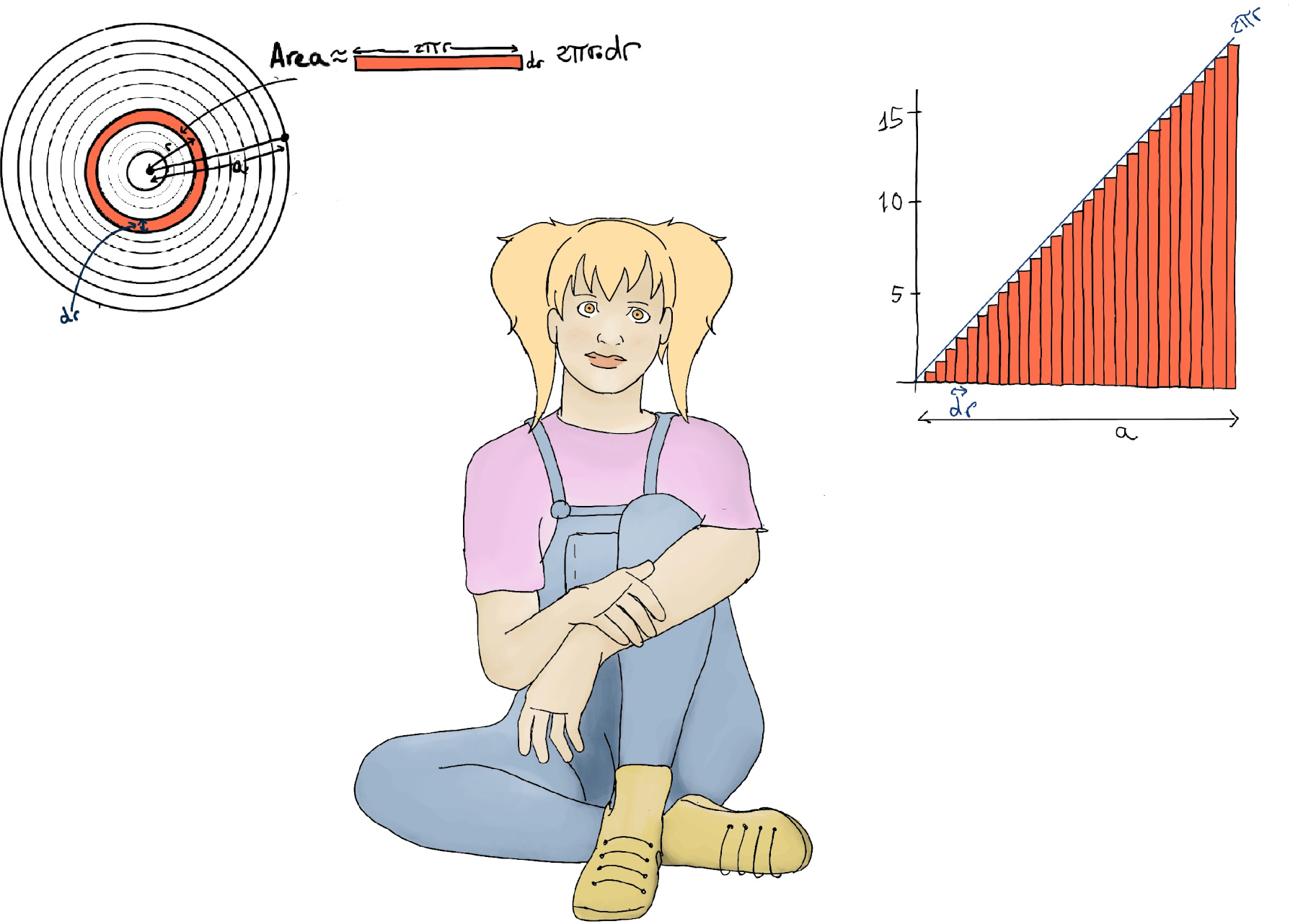
How to calculate the area of a circle of radius a? The best approximation is slicing the circle into many concentric rings. We can approximate the area of any of these concentric rings by 2πr·dr. So we can approximate the area of the whole circle by the sum of these areas (their values of r ranges from “0” to “a” spaced out by dr). This approximation gets more accurate as the size of dr gets smaller and smaller.

We can plot these areas and have a triangle with a base of “a” and a height that is 2π·a, so its area is $\frac{1}{2}·base·height = \frac{1}{2}·a·(2π·a) = π·a^2$

Futhermore, the sum of these rectangles approximates the area under the graph 2πr. More formally, $\int_{0}^{a} 2πrdr = 2π\int_{0}^{a} rdr = 2π\frac{r^2}{2} \bigg|_{0}^{a} = 2π\frac{a^2}{2}-2π\frac{0^2}{2}= π·a^2.$  

Definite integral

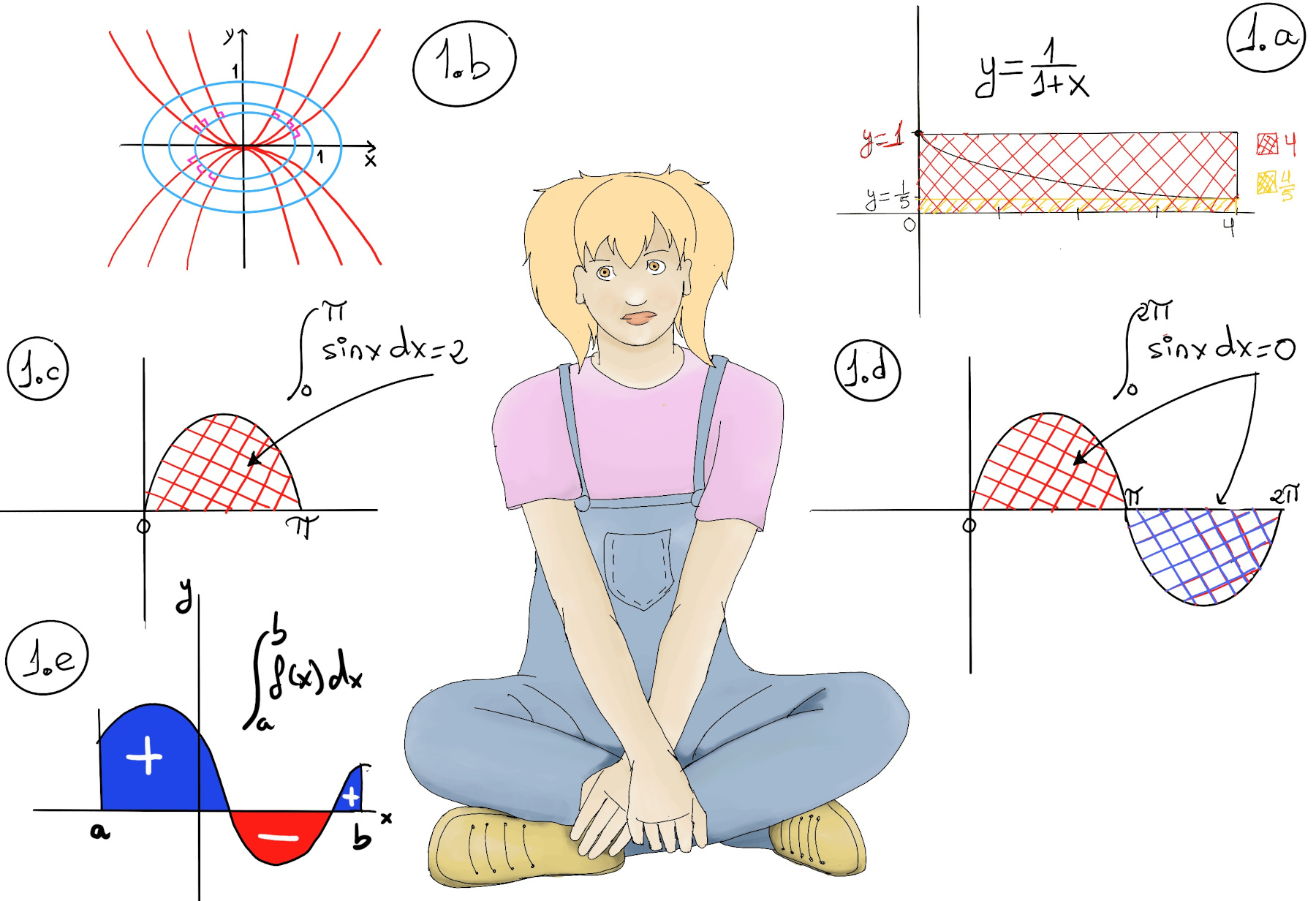
A definite integral is a mathematical concept used to find the area under a curve between two fixed limits. It is represented as $\int_{a}^{b}f(x)dx$, where a and b are the lower and upper limits, and f(x) is the integrand.

A definite integral of a function is defined as the area of the region bounded by the function's graph or curve between two points, say a and b, and the x-axis. The integral of a real-valued function f(x) on an interval [a, b] is written or expressed as $\int_{a}^{b} f(x)dx$ and it is illustrated in Figure 1.a.

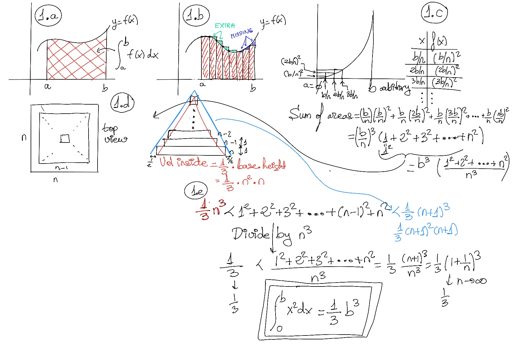
To compute the area, we can divide the region under the function into a series of rectangles whose areas corresponds to function values as heights that are multiplied by the step width to calculate the total sum. Of course, we need to rectify this sum (it is just an approximation) by taking a limit, and as the rectangles get infinitesimally thin, we achieve the desired result (Figure 1.b.).

Let’s try to calculate $\int_{0}^{b} x^2dx$ where a = 0 and b is arbitrary. We divide the segment [0, b] into n pieces (Figure 1.c.). The sum of the areas of all rectangles is equal to $(\frac{b}{n})·(\frac{b}{n})^2+(\frac{b}{n})·(\frac{2b}{n})^2+(\frac{b}{n})·(\frac{3b}{n})^2+···+(\frac{b}{n})·(\frac{nb}{n})^2 = b^3(\frac{1^2+2^2+3^2+···n^2}{n^3})$

To try to understand ${1^2+2^2+3^2+···n^2}$, we can observe that it is basically a pyramid, the base of which is n x n blocks. On top of it, we put a second layer of n-1 x n-1 blocks (Figure 1.d). And we keep on piling up layer after layer. At the top of the pyramid, there is just one block of stone. Underneath our staircase pyramid, there is an ordinary pyramid, and its volume is $\frac{1}{3}(baselength~ ·~ baseheight)·height=\frac{1}{3}n^2~ ·~ n$ On the outside, there is also another ordinary pyramid, with base_length, base_height, and height (n+1), (n+1), and (n+1) respectively.

So our initial quantity ${1^2+2^2+3^2+···n^2}$ is to be found or bounded between these two pyramids: $\frac{1}{3}n^3 < 1^2+2^2+3^2+···n^2 < \frac{1}{3}(n+1)^3$ (Figure 1.e.) If we divide by n³, $\frac{1}{3} < \frac{1^2+2^2+3^2+···n^2}{n^3} < \frac{1}{3}(1+\frac{1}{n})^3$. When n→ infinite, the left and right side tends to $\frac{1}{3}$, and by the Squeeze Infinite, $\frac{1^2+2^2+3^2+···n^2}{n^3} → \frac{1}{3}$ Therefore, our total area $\int_{0}^{b} x^2dx=\frac{1}{3}b^3.$

A Riemann sum is another approximation of an integral by a finite sum. The interval is partitioned into n pieces and we pick any height of f in each interval (e.g. f(c_i)) The sum is defined as $\sum_{i=1}^n f(c_i)\Delta x,~ where~\Delta x=\frac{b-a}{n}$ Please notice that in the limit, as the rectangles get thinner and thinner, the difference between the area covered by the rectangles and the area under the curve will get smaller and smaller, and finally it does not matter our choices (c_i), we get the desired result, that is, $\int_{a}^{b} f(x)dx$.

• Example: Cumulative Debt. Let t be time in years and f(t) be the borrowing rates (euros/years). If we are borrowing money every day, then $\Delta t=\frac{1}{365}.$ The borrowing rate varies over the year. On Day 7 (t=7/365), we borrowed $f(\frac{7}{365})\Delta t = f(\frac{7}{365})\frac{1}{365}$ where f(t) is measured in euros per year, and $\Delta t$ is measured in years, the multiplication is a number of euros that you actually borrow on that very day.

How much money do we borrow in the whole year? $\sum_{i=1}^{365} f(\frac{i}{365})\Delta t$ → [It is going to be very close] $\int_{0}^{1} f(t)dt$

How much money do you actually owe? Obviously, and regretfully, the interest on our debt is compounded continuously. If P is our principal (we start with a debt of P), then after some time t you owe Pe^rt where r is the interest rate.

Compound interest is an interest calculated on both the principal and the existing interest over a given period of time. Its formula is $P(1 +\frac{r}{n})^{nt}$ where n is the number of terms the initial amount or principal P is compounding in the time t. If our debt is compounded continuously, then after time we owe $\lim_{n \to ∞} P(1 + \frac{r}{n})^{nt}=Pe^{rt}$ and we are using the fact that $\lim_{n \to ∞} (1 + \frac{r}{n})^{n} = e^r$.

So, you borrow these amounts $f(\frac{i}{365})\Delta t$, but when you borrow these quantities, the amount of time left in the year is 1 -i/365, which is the amount of time this incremental debt will accumulate interest, that is, $(f(\frac{i}{365})\Delta t)e^{r(1-\frac{i}{365})}$. An at the end of the year, $\sum_{i=1}^{365} (f(\frac{i}{365})\Delta t)e^{r(1-\frac{i}{365})}$ that is basically $\int_{0}^{1} e^{r(1-t)}f(t)dt$.

Fundamental Theorem of Calculus

The Fundamental Theorem of Calculus states roughly that the integral of a function f over an interval is equal to the change of any antiderivate F (F'(x) = f(x)) between the ends of the interval, i.e., $\int_{a}^{b} f(x)dx = F(b)-F(a)=F(x) \bigg|_{a}^{b}$

Examples:

• $\int_{0}^{2} (x^2 +1)dx= (\frac{1}{3}x^3+x)\bigg|_{0}^{2} = (\frac{1}{3}2^3+2)-(\frac{1}{3}0^3+0) = \frac{14}{3}$.
• $\int_{0}^{3} x^2+4dx=(\frac{1}{3}x^3 + 4x)\bigg|_{0}^{3}=(\frac{1}{3}·3^3+4·3)-(\frac{1}{3}·0^3+4·0) =21$.
• $\int_{0}^{π} sinxdx = (-cosx)\bigg|_{0}^{π}=-cosπ-(-cos0) = -(-1)-(-1) = 2$.
• $\int_{0}^{\frac{π}{4}} sin(2x)dx = \frac{-1}{2}cos(2x)\bigg|_{0}^{\frac{π}{4}} = -\frac{1}{2}cos(2·\frac{π}{4}) +\frac{1}{2}cos(2·0) = -\frac{1}{2}·0 + \frac{1}{2}·1 = \frac{1}{2}.$
• $\int_{0}^{\frac{π}{2}} sin(x)cos(x)dx$ =[Recall the double-angle indentity for sine, sin(2x) = 2sin(x)cos(x)] = $\frac{-1}{4}cos(2x)\bigg|_{0}^{\frac{π}{2}} = \frac{-1}{4}cos(2·\frac{π}{2}) + \frac{1}{4}cos(2·0) = \frac{-1}{4}·(-1) + \frac{1}{4} = \frac{1}{2}.$
• $\int_{0}^{1} x^4dx =\frac{x^5}{5}\bigg|_{0}^{1}=\frac{1}{5}$
• Find the total area between f(x) = x -2 and the x-axis over the interval [0, 6] (Figure 1)  

1. Calculate the x-intercept of f(x): (2, 0).
2. Total area = Area below the x-axis over the subinterval [0, 2] (A₂) + Area above the x-axis over the subinterval [6, 2] (A₁). $\int_{0}^{6} |f(x)| = A_2 + A_1$
3. Using basic trigonometry, $A_2 = \frac{1}{2}bh = \frac{1}{2}·2·2 = 2, A_1 = \frac{1}{2}·4·4 = 8$ ⇒ A = 2 + 8 = 10.

• By using a definite integral find the area of the region bounded by y = x and y = $3\sqrt{x}$ (Figure 3).  

1. First, we need to find the points of intersection between these two curves. $x = 3\sqrt{x}↭x^2 = 9·x↭ x(x-9) = 0 ↭ $ x = 0 and 9
2. Then, we integrate the difference between the upper and lower curves over that interval, $\int_{0}^{9} (3\sqrt{x}-x)dx = 3·\frac{x^{\frac{3}{2}}}{\frac{3}{2}} -\frac{x^2}{2}\bigg|_{0}^{9} = 2·9^{\frac{3}{2}} -\frac{81}{2} = 13.5.$

• By using a definite integral find the area of the region bounded by y = 6x -x² and y = 0 (Figure 2).  

1. Calculate the x-intercepts of f(x) = 6x -x² and the x-axis, 6x -x² = x(6-x) = 0 ⇒ the x-intercepts are (0, 0) and (6, 0).
2. Total area = Area above the x-axis between 0 and 6. $\int_{0}^{6} 6x -x^2 = 3x^2 -\frac{1}{3}x^3\bigg|_{0}^{6} = 3·6^2 -\frac{1}{3}6^3 - (3·0^2 -\frac{1}{3}·0^3) = 36.$

Intuitive interpretation of Fundamental Theorem

For some distance s(t), the velocity function is v(t)=s’(t). Therefore, given a velocity function, v(t) (v(t) is what is measured in the speedometer), $\int_{a}^{b} v(t)dt$ =s(b)-s(a) where s(b) - s(a) is the actual distance traveled, that is, what is measured in the odometer, that is, the instrument on your car dashboard that displays how many miles or kilometers your vehicle has traveled.

Let’s say that you checked your speedometer every single second (Is your phone out of juice? 😃. Seriously, $\Delta t = 1~ second$), $v(t_i)\Delta t$ is the distance traveled in the ith second, the Riemman Sum is equal $\sum_{i=1}^n v(t_i)\Delta t≈\int_{a}^{b} v(t)dt$ = s(b)-s(a) -how far you have traveled-.

Reality is always a little more complex

Let’s notice that $\int_{0}^{2π} sinxdx = (-cosx)\bigg|_{0}^{2π}=-cos2π-(-cos0) = -1 -(-1) = 0$ (Figure 1.d.)

💡A definite integral of a function should be interpreted as the signed area of the region in the plane that is bounded by its graph and the horizontal axis. Be extremely careful, areas above the horizontal -x- axis of the plane are positive while areas below the horizontal axis are considered negative (Figure 1.e.).

Bibliography

1. NPTEL-NOC IITM, Introduction to Galois Theory.
2. Algebra, Second Edition, by Michael Artin.
3. LibreTexts, Calculus. Abstract and Geometric Algebra, Abstract Algebra: Theory and Applications (Judson).
4. Field and Galois Theory, by Patrick Morandi. Springer.
5. Michael Penn, and MathMajor.
6. Contemporary Abstract Algebra, Joseph, A. Gallian.
7. YouTube’s Andrew Misseldine: Calculus. College Algebra and Abstract Algebra.
8. MIT OpenCourseWare 18.01 Single Variable Calculus, Fall 2007 and 18.02 Multivariable Calculus, Fall 2007.
9. Calculus Early Transcendentals: Differential & Multi-Variable Calculus for Social Sciences.