Concavity and inflection points

When lies spread like wildfire, money, power, and pleasure are worshipped as God in the midst of a post-modern identity crisis where “the self” has become the center of the universe and decides what is right or wrong, so moral is subjective, societies fall apart and violence reigns, Anawim, #justtothepoint.

Recall

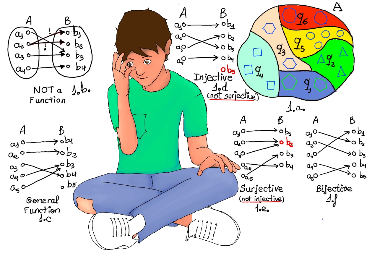
Definition. A function f is a rule, relationship, or correspondence that assigns to each element of one set (x ∈ D), called the domain, exactly one element of a second set, called the range (y ∈ E).

The pair (x, y) is denoted as y = f(x). Typically, the sets D and E will be both the set of real numbers, ℝ.

Graphing functions involves the visual representation of a curve that reflects the behavior of a mathematical function on a coordinate plane, also known as the Cartesian plane. It is a two-dimensional space defined by two axes - the x-axis (horizontal) and the y-axis (vertical).

A systematic approach to graphing a function begins by constructing a table containing selected input values and their corresponding output values. By extending this table, we can plot the points on the coordinate plane and observe the pattern they form. Connecting these points reveals the shape of the curve, allowing us to gain insights into the behavior of the function across its domain. This process provides a visual means of understanding the relationships between different variables and aids in interpreting the overall characteristics of the function.

Concave Functions

Concavity and inflection points are essential concepts in calculus that describe the curvature of functions. Understanding concavity and identifying inflection points provides valuable insights into the behavior of functions.

The concavity of a function is the direction in which the function opens. If it opens upwards, it is called concave up. Otherwise, it is called concave down.

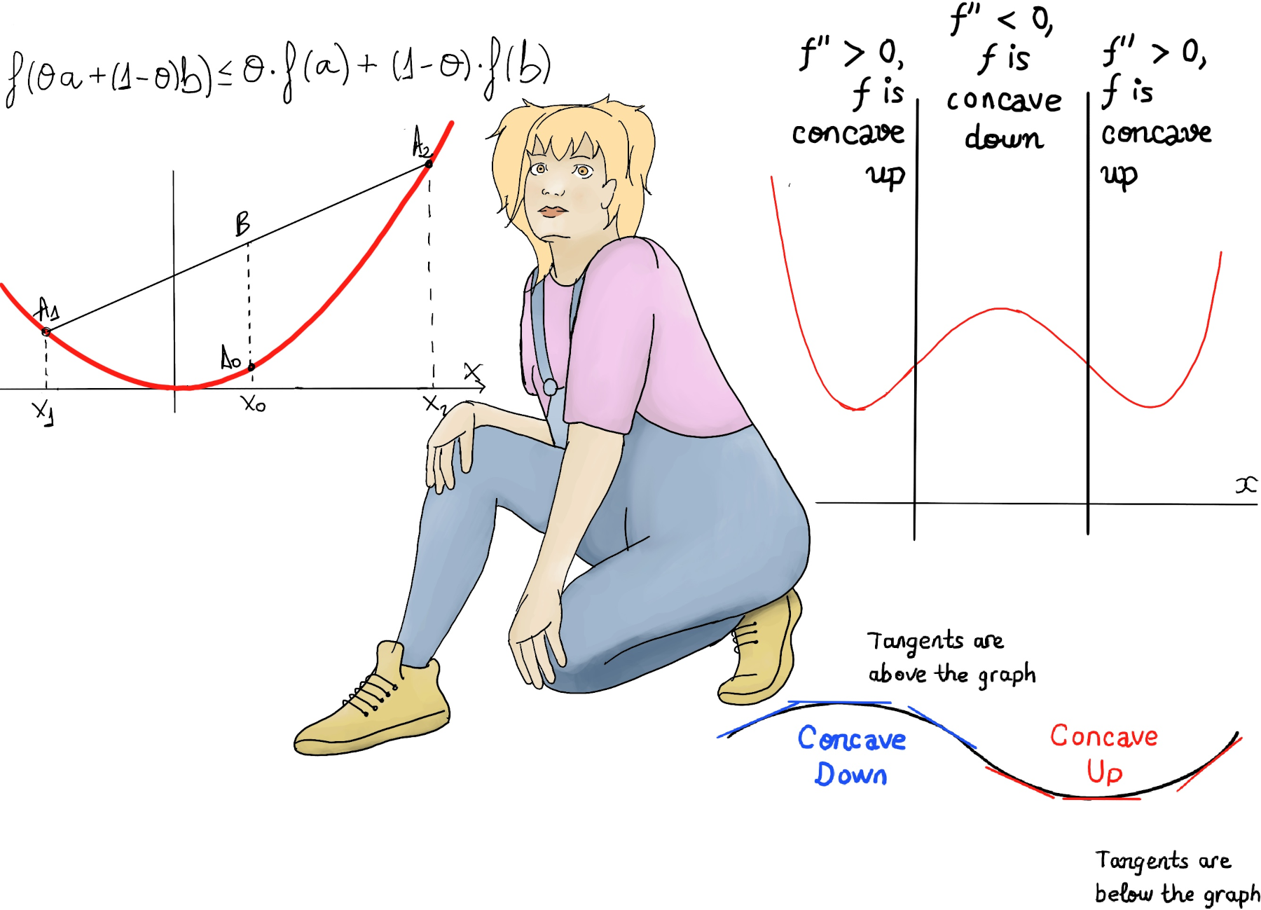
Definition. A function is concave up or convex if it curves or bends upwards, the line segment or chord between any two points A₁, A₂, on the graph of the function, lies above the graph between the two points (the midpoint B lies above the corresponding point A₀ of the graph of the function). It means that the function's graph is shaped like a 'U', a bowl, or a smiley face 😃 and lies above its tangent lines on that interval.

Definition. A function is concave down or just concave if it curves or bends downwards. It means that the function's graph is shaped like an upside-down 'U', i.e., '∩', an umbrella, or a frowny face 😞 and lies below its tangent lines on that interval.

Formally, f is concave up or convex on an interval [a, b] if ∀ x₁, x₂ ∈ [a, b], ∀θ such that 0 < θ <1, the following inequality holds: f(θa + (1-θ)b) ≤ θf(a) + (1-θ)f(b) where θa + (1-θ)b ∈ (a, b). f is concave down on an interval [a, b] if ∀ x₁, x₂ ∈ [a, b], ∀θ such that 0 < θ <1, the following inequality holds: f(θa + (1-θ)b) ≥ θf(a) + (1-θ)f(b) where θa + (1-θ)b ∈ (a, b).

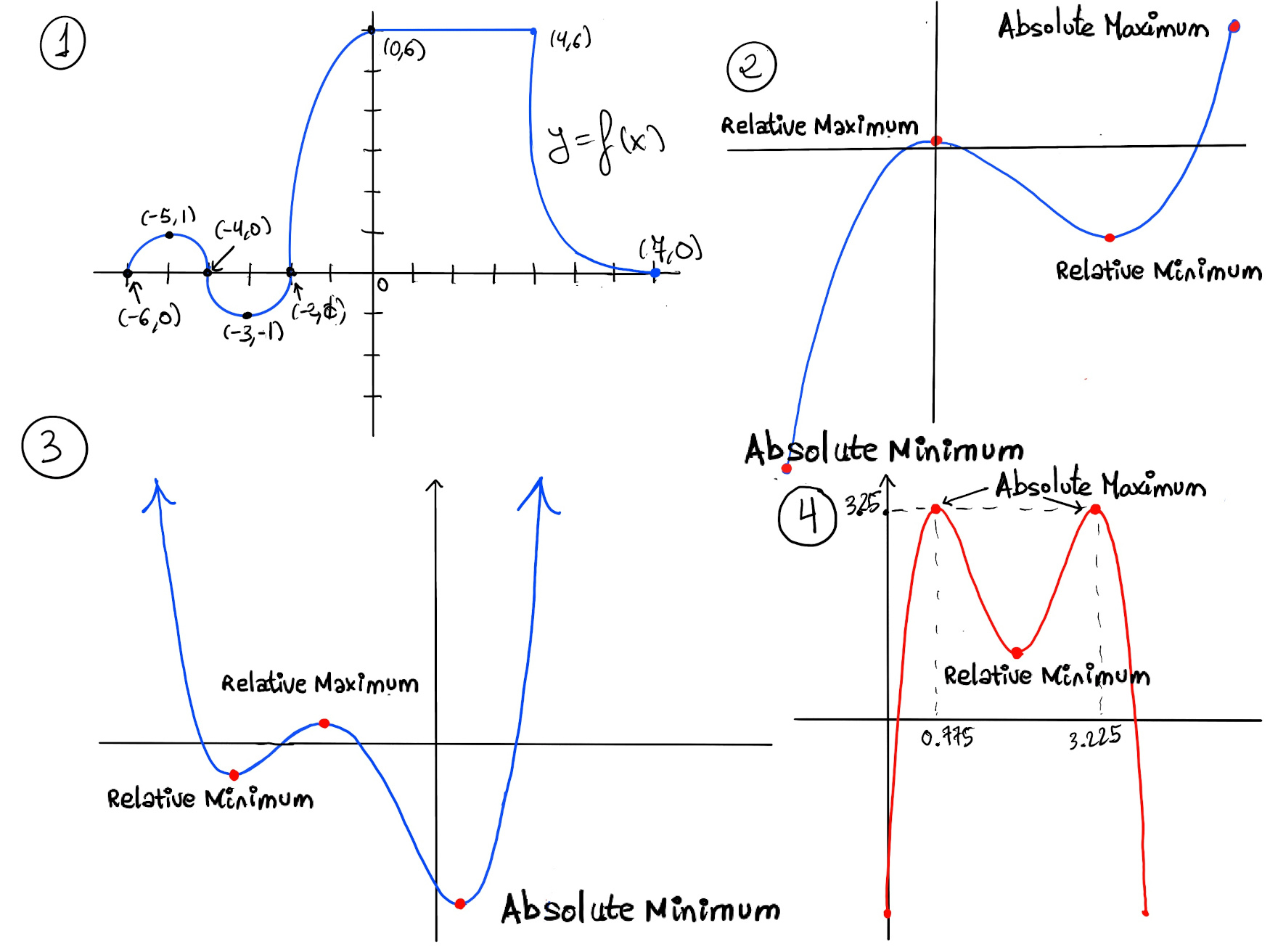
The function f (Figure 1) is increasing on (-6, -5) ∪ (-3, 0) and decreasing on (-5, -3) ∪ (4, 7). It is constant on [0, 4]. Futhermore, f is concave up on (-4, -2) ∪ (4, 7) and concave down on (-6, -4) ∪ (-2, 0).

The equation of a parabola is y = ax² + bx + c, where a, b, and c are constants. The parabola is a classic example of a concave up curve or convex when a is positive. It is a symmetrical curve that has a U-shape. If a is negative, the curve will be concave down or just concave.

Concavity relates to the rate of change of a function’s derivative. A function is concave up or convex if its derivative f' is increasing, that is, its second derivate f'' is positive. Similarly, f is concave down or concave where its derivative f' is decreasing or equivalently, its second derivate f'' is negative.

Since the second derivative of any quadratic function is just 2a, the sign of a directly correlates with the concavity of the function. If a is positive, 2a is positive so the function is concave up, e.g., x² -Figure ii-, 3x² - 4x + 4. If a is negative, 2a is negative so the function is concave down, e.g., -x² -Figure ii-, -3x² + 4x + 4.

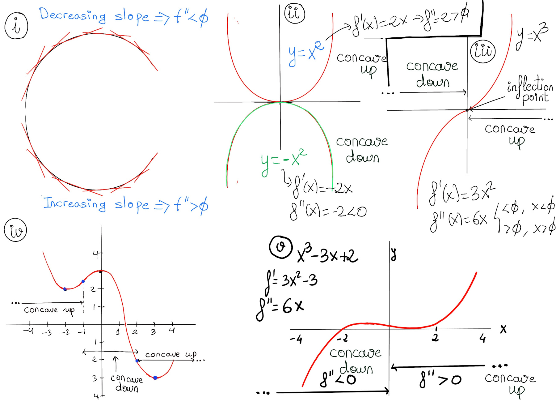
An inflection point is a point at which the curvature changes sign, i.e., where the function changes from being concave up to concave down or viceversa.The graph of a differentiable function has an inflection point at (x, f(x)) if and only if its first derivative f’ has an isolated extremum (a local minimum or maximum) at x. In other words, if a function second derivative f″(x) exists at x₀ and x₀ is an inflection point for f, then f″(x₀) = 0.

However, it’s important to emphasize that not all points where the second derivative is zero or undefined are inflection points. The concavity must change at these points for them to be considered inflection points.

Solved examples

• f(x) = x² (Figure ii), f’(x) = 2x, f’’(x) = 2 > 0, f is concave up.
• f(x) = -x² (Figure ii), f’(x) = -2x, f’’(x) = -2 < 0, f is concave down.
• f(x) = x³ (Figure iii), f’(x) = 3x², f’’(x) = 6x.

1. x > 0 ⇒ f’’(x) > 0, f is concave up.

2. x < 0 ⇒ f’’(x) < 0, f is concave down.

3. 0 is an inflection point.

   f(x) = $\frac{1}{x}, f’(x)=\frac{-1}{x^2}, f’’(x)=\frac{2}{x^3}$ has the same behaviour, but 0 is not an inflection point due to the fact that f is undefined at x = 0.

• f(x) = x³-3x+2 (Figure v), f’(x) = 3x²-3, f’’(x) = 6x.

1. x > 0 ⇒ f’’(x) > 0, f is concave up.
2. x < 0 ⇒ f’’(x) < 0, f is concave down.
3. 0 is an inflection point.

• f(x) = 3x -x³ (Figure 1.e)

f’(x) = 3 -3x², f’’(x) = -6x.

1. x < 0, f’’(x) > 0 ⇒ f’ is increasing ⇒ f is concave up.
2. x > 0, f’’(x) < 0 ⇒ f’ is decreasing ⇒ f is concave down.
3. 0 is an inflection point.

• f(x) = $\frac{x+1}{x+2}$

1. f’(x) = ¹⁄_{(x + 2)²} > 0 ∀x ∈ ℝ, x ≠ -2 ⇒ f is increasing (-∞, -2)∪(-2, ∞).
2. f’’(x) = ^-2⁄_{(x + 2)³}, x < -2 ⇒ f’’(x) > 0, concave upward.
3. x > -2 ⇒ f’’(x) < 0, concave downward.
4. -2 is not an inflection point because the function is undefined at this value.

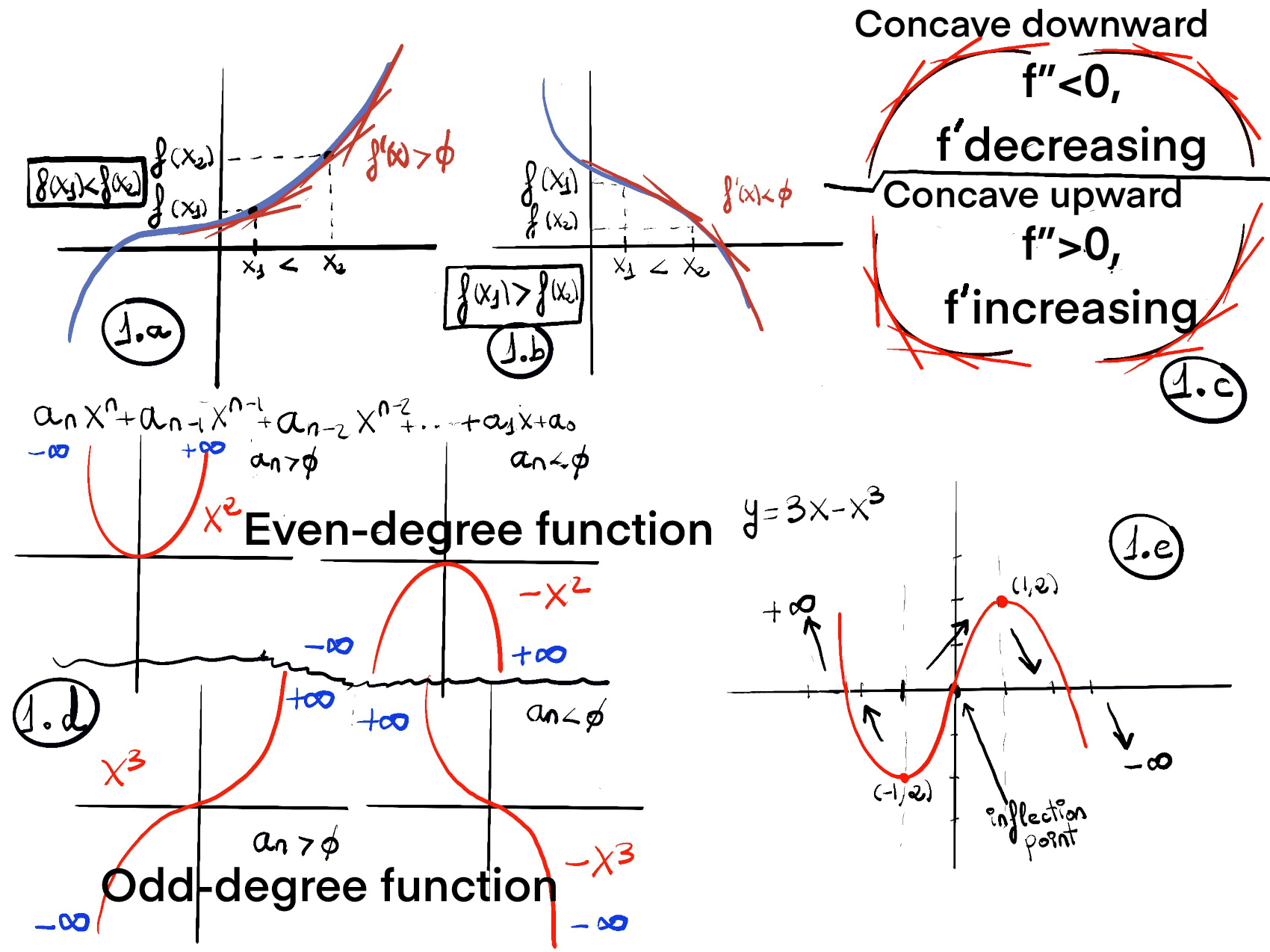
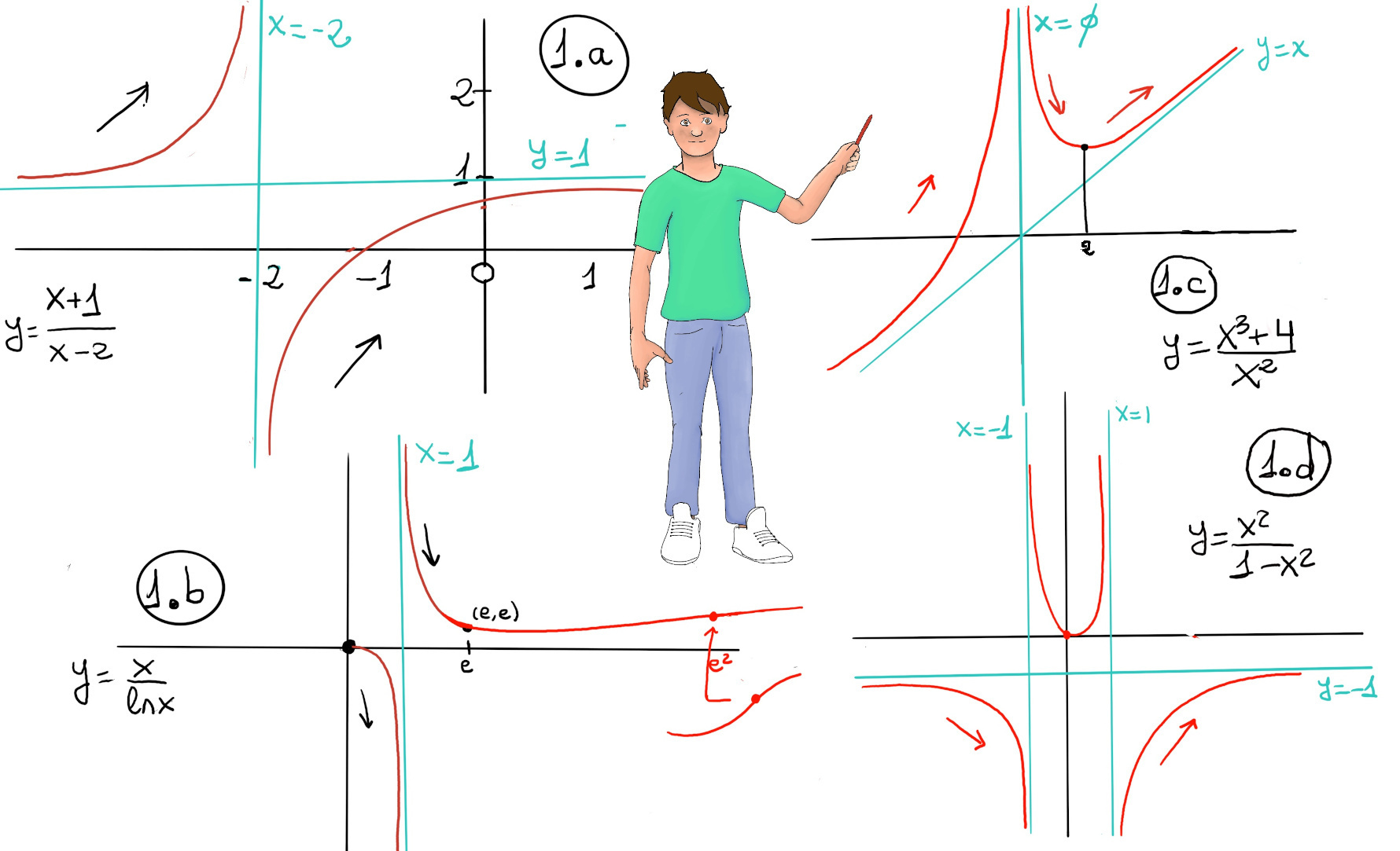
The plot is shown in Figure 1.a.  

More examples because you can never have enough of what you don’t really need 😄.

• f(x)=2x³ −12x² +4x −27, f’(x) = 6x² -24x +4, f’’(x)= 12x -24 = 0 ↭ x = 2.

1. (-∞, 2), e.g., f’’(0) = -24 < 0, f concave down.
2. (2, ∞), e.g., f’’(3) = 36 -24 = 12, f’’(x) > 0, f concave up.
3. 2 is an inflection point.

• f(x) = sin(x) + cos(x), Domain(f) = [0, 2π]. f’(x) = cos(x) -sin(x), f’’(x) = -sin(x) -cos(x), f’’(x) = 0 ↭ -sin(x) = cos(x) ⇒ x = $\frac{π}{2}+\frac{π}{4} = \frac{3π}{4}$ and $\frac{3π}{4} + π = \frac{7π}{4}$ ($\frac{π}{4}$ in the Q2, Q4 quadrants of the Cartesian system).

1. (0, $\frac{3π}{4}$), e.g., f’’($\frac{π}{2}$) = -1 < 0, f concave down.
2. ($\frac{3π}{4}, \frac{7π}{4}$), e.g., f’’(π) = 1, f’’(x) > 0, f concave up.
3. ($\frac{7π}{4}, 2π$), e.g., f’’($\frac{11π}{6}$) = -0.366, f’’(x) < 0, f concave down.
4. $\frac{3π}{4}, \frac{7π}{4}$ are points of inflections.

• f(x) = $\frac{x^{2}}{1-x^{2}}$

1. Domain = ℝ - {1, -1}. f(0) = 0.
2. f’(x) = $\frac{2x}{(1-x^{2})^{2}}$. Critical points: 0 (f’(x)=0), 1 and -1 (f’ is undefined). x < -1, f’(x) < 0 ⇒ f decreasing ↘. -1 < x < 0, f’(x) < 0 ⇒ f decreasing ↘. 0 < x < 1, f’(x) > 0 ⇒ f increasing ↗. x > 1, f’(x) > 0 ⇒ f increasing ↗.
3. f’’(x) = $\frac{6x^{2}+2}{(1-x^{2})^{3}}$. x < -1, f’’(x) < 0 ⇒ concave down
   -1 < x < 1, f’’(x) > 0 ⇒ concave up
   x > 1, f’’(x) < 0 ⇒ concave down
4. 1 and -1 are not inflection points because f is undefined at these points.

The plot is shown in Figure 1.d.  

• f(x) = ^x⁄_lnx, x > 0.

Dom(f) = ℝ⁺ - {0, 1}.

f’(x) = $\frac{lnx-x(\frac{1}{x})}{(lnx)^{2}}=~ \frac{lnx -1}{(lnx)^{2}}$

f’(x) = 0 ↭ lnx = 1 ↭ x = e, and f(e) = e.

Futhermore: If 0 < x < 1, f’(x) < 0 ⇒ f is decreasing ↘. 1 < x < e, f’(x) < 0 ⇒ f is decreasing ↘. x > e, f’(x) > 0 ⇒ f is increasing ↗. Hence, f has a local minimum at x = e.

Let’s calculate f’’(x) = $\frac{\frac{1}{x}(lnx)^{2}-\frac{(lnx-1)2lnx}{x}}{(lnx)^{4}}=~ \frac{\frac{lnx-2(lnx-1)}{x}}{(lnx)^{3}}=~ \frac{2-lnx}{x(lnx)^{3}}$

Therefore, 0 < x < 1, f’’(x) < 0 ⇒ concave down. 1 < x < e², f’(x) > 0 ⇒ concave up. x > e², f’(x) < 0 ⇒ concave down. e² is an inflection point, a point where concavity changes. The plot is shown in Figure 1.b.

Bibliography

1. NPTEL-NOC IITM, Introduction to Galois Theory.
2. Algebra, Second Edition, by Michael Artin.
3. LibreTexts, Calculus. Abstract and Geometric Algebra, Abstract Algebra: Theory and Applications (Judson).
4. Field and Galois Theory, by Patrick Morandi. Springer.
5. Michael Penn, and MathMajor.
6. Contemporary Abstract Algebra, Joseph, A. Gallian.
7. YouTube’s Andrew Misseldine: Calculus. College Algebra and Abstract Algebra.
8. MIT OpenCourseWare 18.01 Single Variable Calculus, Fall 2007 and 18.02 Multivariable Calculus, Fall 2007.
9. Calculus Early Transcendentals: Differential & Multi-Variable Calculus for Social Sciences.