Vector fields

Quantity has a quality of its own, Joseph Stalin.

Vector fields

A vector field is, roughly speaking, an assignment of a vector $\vec{F}$ to each point (x, y) in a space, i.e., $\vec{F} = M\vec{i}+N\vec{j}$ where M and N are functions of x and y.

Vector fields are commonly used to model physical phenomena, such as the speed and direction of a moving fluid (like wind speed -meters/seconds-) or the strength and direction of forces (such as magnetic or gravitational forces) as they vary across space.

A vector field on a plane can be visualized as a collection of arrows, each attached to a point on the plane. These arrows represent vectors with specific magnitudes and directions.

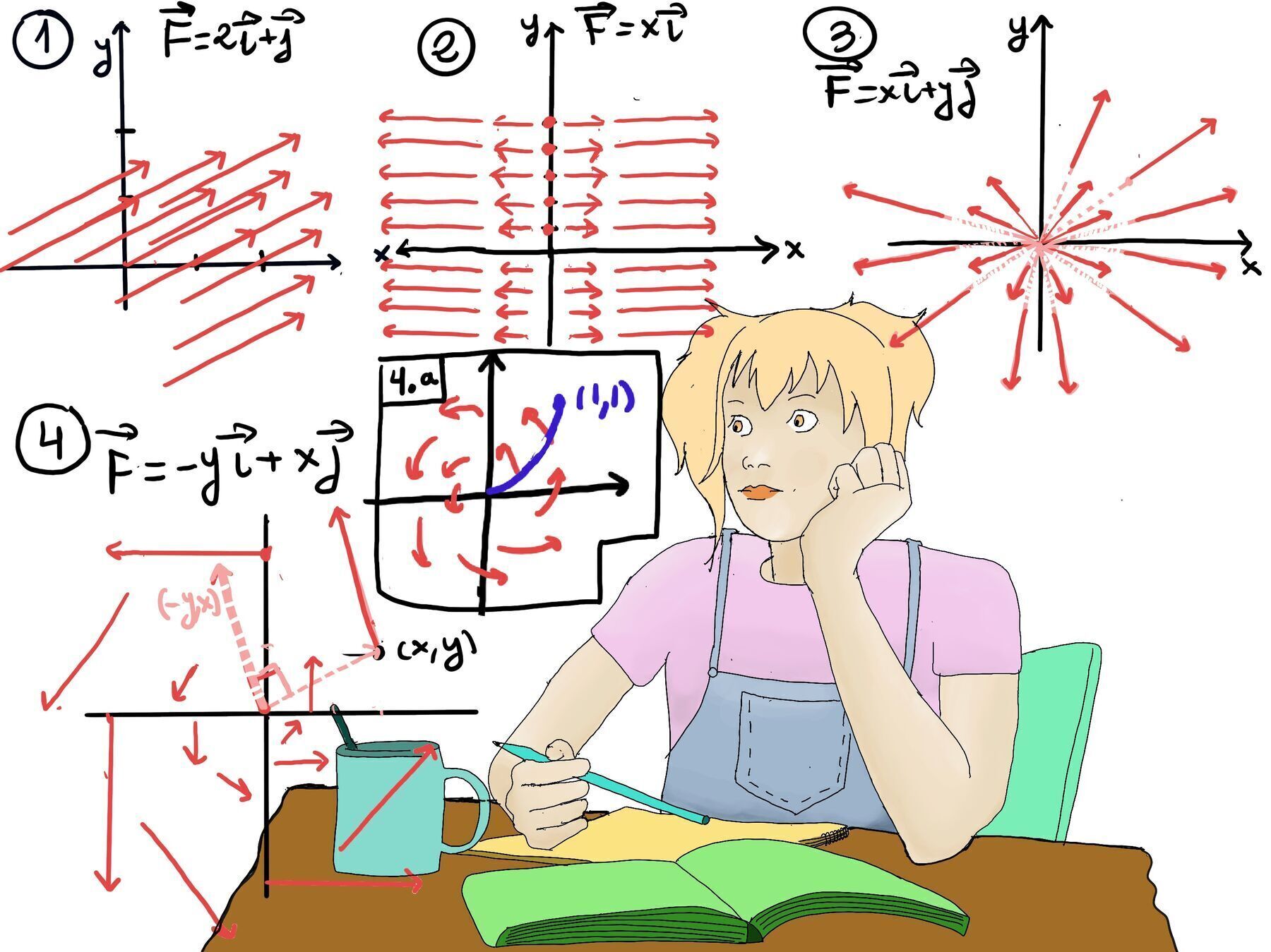
We are going to illustrate the following vector fields: $\vec{F} = 2\vec{i}+\vec{j}$ (Figure 1, the vector does not depend on x and y), $\vec{F} = x \vec{i}$ (Figure 2), $\vec{F} = x\vec{i}+y\vec{j}$ (Figure 3), and $\vec{F} = -y\vec{i}+x\vec{j}$ (Figure 4, (x, y)→(-y,x), i.e., 90° counter-clockwise).

Work and line integrals

In its simplest form, for a constant force aligned with the direction of motion, the work equals the product of the force strength and the distance traveled, W = force · distance = $\vec{F}·Δ\vec{r}$.

More generally, work is the energy transferred when a force acts on an object and displaces it along a path. In the context of vector fields, we can calculate the work done by a force field along a curve or trajectory C, W = $\int_{C} \vec{F}·d\vec{r}$ (= $\lim_{\Delta r_i \to 0} \sum_{i} \vec{F}·Δ\vec{r_i} = \lim_{\Delta r_i \to 0} \sum_{i} \vec{F}·\frac{Δ\vec{r_i}}{Δt}·Δt$, realize that $\frac{Δ\vec{r_i}}{Δt}$ is the velocity vector)

Therefore, W = $\lim_{\Delta t \to 0}\sum_{i} (\vec{F}·\frac{Δ\vec{r_i}}{Δt}·Δt)$ ⇒ W = $\int_{C} \vec{F}·d\vec{r} = \int_{t_1}^{t_2} (\vec{F}·\frac{d\vec{r}}{dt}·dt)$

• Exercise. Let $\vec{F} = -y\vec{i}+x\vec{j}$, and the curve x = t, y = t², 0 ≤ t ≤ 1 (Figure 4.a, C is the blue parabola).

W = $\int_{C} \vec{F}·d\vec{r} = \int_{t_1}^{t_2} (\vec{F}·\frac{d\vec{r}}{dt}·dt) = \int_{0}^{1} (\vec{F}·\frac{d\vec{r}}{dt}·dt)$

Consider $\vec{F} = ⟨-y, x⟩ =$[x = t, y = t²] = ⟨-t², t⟩. Besides, $\frac{dx}{dt}=1,\frac{dy}{dt}= 2t, \frac{d\vec{r}}{dt}=⟨1,2t⟩$

W = $\int_{0}^{1} (\vec{F}·\frac{d\vec{r}}{dt}·dt) =\int_{0}^{1} ⟨-t^2, t⟩ ⟨1, 2t⟩ dt = \int_{0}^{1} (-t^2+2t)dt = \int_{0}^{1} t^2dt = \frac{t^3}{3}\bigg|_{0}^{1} = \frac{1}{3}$

Another way of putting it, $\vec{F} = ⟨M, N⟩, \vec{dr} = ⟨dx, dy⟩ ⇒ \vec{F}·\vec{dr} = ⟨M, N⟩ · ⟨dx, dy⟩ = Mdx + Ndy$

W = $\int_{C} \vec{F}·d\vec{r} = \int_{C} Mdx + Ndy$

Evaluating Double Integrals

A method to evaluate double integrals is to express x and y in terms of a single variable, then substitute, and finally integrate.

Let $\vec{F} = -y\vec{i}+x\vec{j}$, and the curve x = t, y = t², 0 ≤ t ≤ 1 ⇒ dx = dt, dy = 2t·dt.

W = $\int_{C} \vec{F}·d\vec{r} = \int_{C} Mdx + Ndy = \int_{C} -t^2dt+t·2tdt = \int_{0}^{1} t^2dt = \frac{1}{3}.$

This method depends on the trajectory C, but not on parametrization, e.g., the previous example, we could have chosen x = sin(θ), y = sin(θ), 0 ≤ θ ≤ $\frac{π}{2}$.

Geometrical interpretation

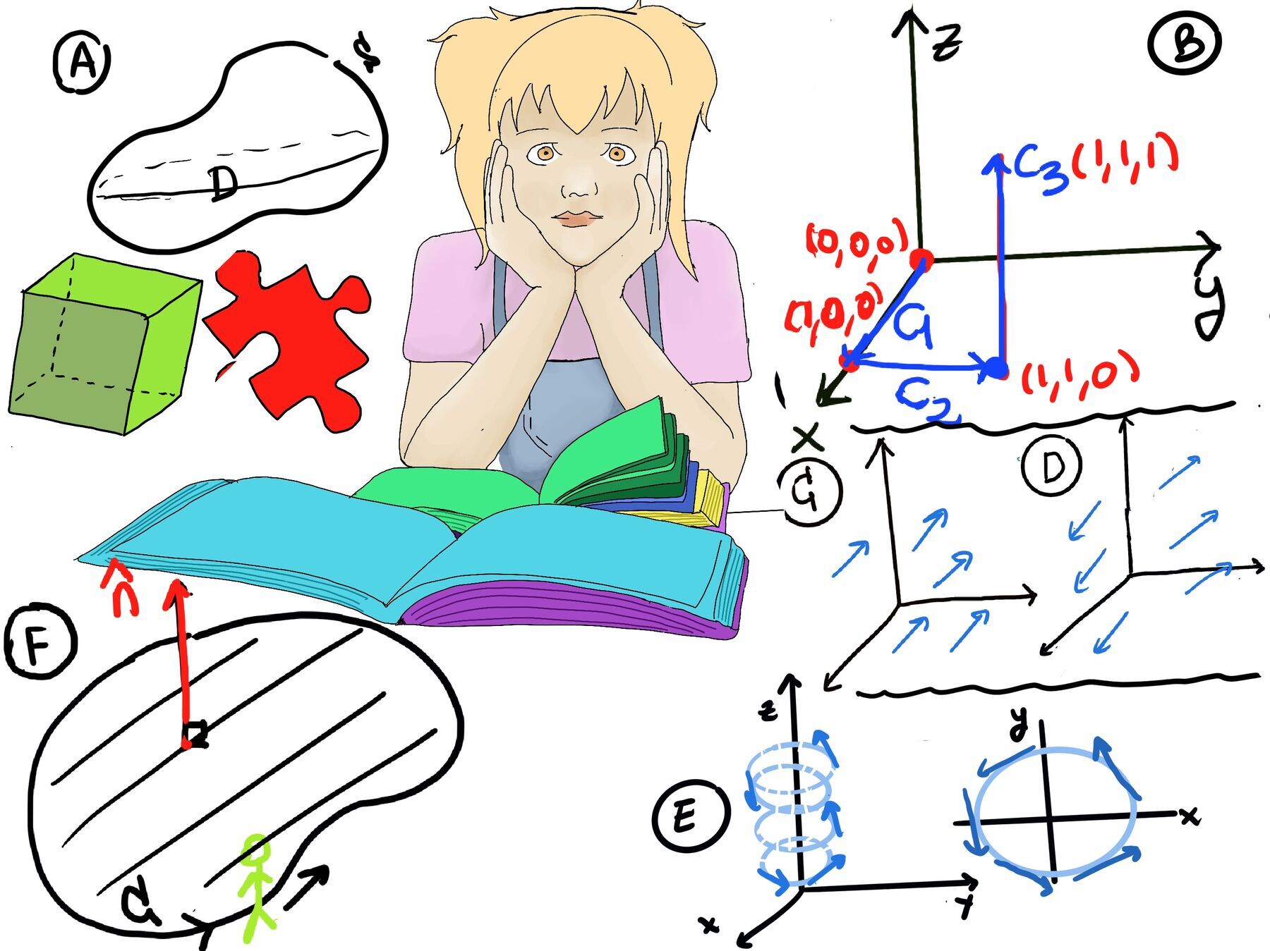
Recall that the unit tangent vector $\hat{\mathbf{T}}$ is a normalized vector (it has a length of one) that is tangent to a curve at any point. It is a vector that points in the direction of the curve’s movement as it passes through that point.

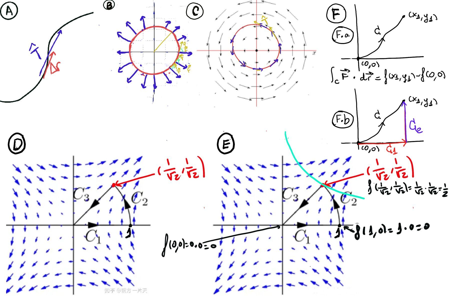
If a take a small piece of our trajectory C, $Δ\vec{r}$, it will go in the same direction as the unit vector and its length is Δs (s is the distance along the trajectory), that is, $d\vec{r} = ⟨dx, dy⟩ = \hat{\mathbf{T}}·ds$ (ds is the arclength) -Figure A.-

Therefore, W = $\int_{C} \vec{F}·d\vec{r} = \int_{C} \vec{F}·\hat{\mathbf{T}}·ds$

• Let C be a circle of radius “a” at origin counterclocwise, $\vec{F} = x\vec{i} + y\vec{j}$, compute the work done by the force as we move along C. Geometrically, we can see that the work is zero because the force is perpendicular to the motion (Figure B) ↭ $\vec{F} ⊥\hat{\mathbf{T}}⇒ \vec{F} · \hat{\mathbf{T}} = 0 ⇒\int_{C} \vec{F}·\hat{\mathbf{T}}·ds = 0$.

• Let C be a circle of radius “a” at origin counterclocwise, $\vec{F} = -y\vec{i} + x\vec{j}$ (Figure C), compute the work done by the force as we move along C. Geometrically, we can see that the force is parallel to the motion ↭ $\vec{F} || \hat{\mathbf{T}} ⇒ \vec{F}·\hat{\mathbf{T}} = |\vec{F}| ⇒ \int_{C} \vec{F}·\hat{\mathbf{T}}·ds = \int_{C} |\vec{F}|·ds = \int_{C} a·ds = a\int_{C}ds = a·length(C) = a·2πa = 2πa^2$.

Alternatively, W = $\int_{C} \vec{F}·d\vec{r} = \int_{C} Mdx + Ndy =\int_{C} -ydx +xdy$=[x = acos(θ), y = asin(θ), 0 ≤ θ ≤ 2π ]=$\int_{C} -(asin(θ))(-asin(θ)dθ)+(acos(θ))(acos(θ)dθ = \int_{C} a^2(sin^2(θ)+cos^2(θ)) = \int_{0}^{2π} a^2dθ = a^2\int_{0}^{2π} dθ = a^2·2π$

• Let’s do a more complicated exercise where the vector field is given ($\vec{F}= y\vec{i}+x\vec{j}$ = ⟨x, y⟩) amd we want the work done as we move along C = C₁+ C₂ + C₃ in the unit circle. We are working at the unit disk, so we can tell that 0 ≤ θ ≤ ^π⁄₄ (Figure D)

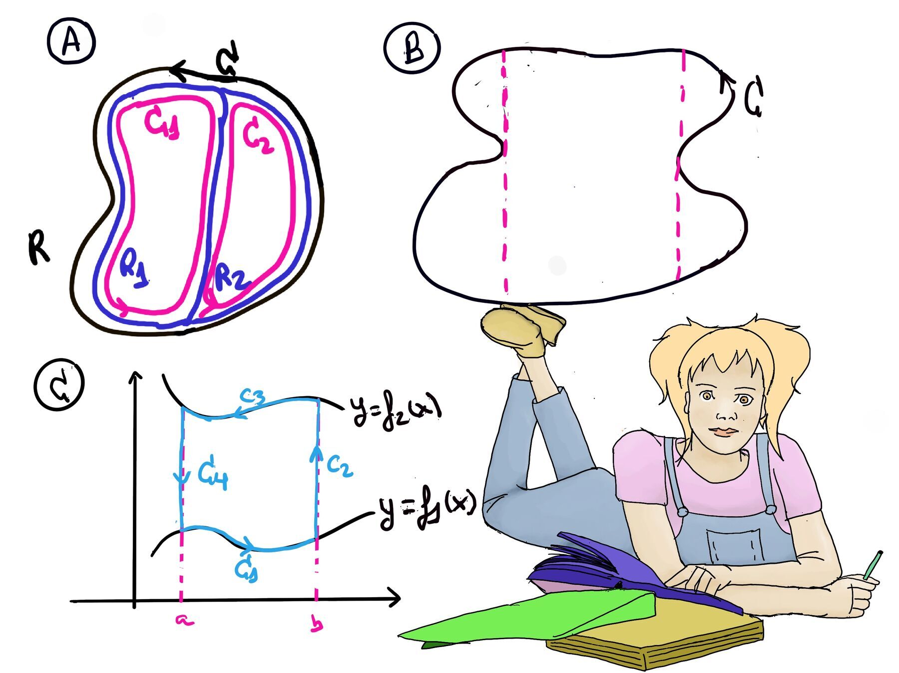
W = $\int_{C} \vec{F}·d\vec{r} = \int_{C_1} \vec{F}·d\vec{r} + \int_{C_2} \vec{F}·d\vec{r} + \int_{C_3} \vec{F}·d\vec{r} = \int_{C_1} (ydx+xdy) + \int_{C_2} (ydx+xdy) + \int_{C_3} (ydx+xdy)$

$\int_{C_1} (ydx+xdy) =$[y = 0 ⇒ dy = 0] $\int_{C_1} (0·dx+x·0) = \int_{C_1} 0 = 0$ (Geometrically, the vector field is perpendicular to the motion).

$\int_{C_2} (ydx+xdy) =$[Notice that C₂ is a portion of the unit circle, so polar coordinates are a good idea, x = cos(θ), y = sin(θ), 0 ≤ θ ≤ ^π⁄₄, dx = -sin(θ)dθ, dy = cos(θ)dθ] =$\int_{C_2} (sin(θ)(-sin(θdθ))+ cos(θ)·(cos(θ)dθ)) = \int_{0}^{\frac{π}{4}} cos^2(θ)-sin^2(θ)dθ = \int_{0}^{\frac{π}{4}} cos(2θ)dθ = \frac{1}{2}sin(2θ)\bigg|_{0}^{\frac{π}{4}} = \frac{1}{2}$

$\int_{C_3} (ydx+xdy) =$ [$x = \frac{1}{\sqrt{2}}-\frac{1}{\sqrt{2}}t, y = \frac{1}{\sqrt{2}}-\frac{1}{\sqrt{2}}t$, 0 ≤ t ≤ 1, but a better idea is x = t, y = t, 0 ≤ t ≤ $\frac{1}{\sqrt{2}}$ and we will get the work backwards ⇒ dx = dy = dt]

$\int_{-C_3} (ydx+xdy) = \int_{0}^{\frac{1}{\sqrt{2}}} tdt+tdt = \int_{0}^{\frac{1}{\sqrt{2}}} 2tdt = t^2\bigg|_{0}^{\frac{1}{\sqrt{2}}} = \frac{1}{2}$

⇒ $\int_{C_3} (ydx+xdy) = -\frac{1}{2} ⇒ W = \int_{C_1} (ydx+xdy) + \int_{C_2} (ydx+xdy) + \int_{C_3} (ydx+xdy) = 0 + \frac{1}{2} -\frac{1}{2} = 0.$

Bibliography

1. NPTEL-NOC IITM, Introduction to Galois Theory.
2. Algebra, Second Edition, by Michael Artin.
3. LibreTexts, Calculus and Calculus 3e (Apex). Abstract and Geometric Algebra, Abstract Algebra: Theory and Applications (Judson).
4. Field and Galois Theory, by Patrick Morandi. Springer.
5. Michael Penn, and MathMajor.
6. Contemporary Abstract Algebra, Joseph, A. Gallian.
7. YouTube’s Andrew Misseldine: Calculus. College Algebra and Abstract Algebra.
8. MIT OpenCourseWare 18.01 Single Variable Calculus, Fall 2007 and 18.02 Multivariable Calculus, Fall 2007.
9. Calculus Early Transcendentals: Differential & Multi-Variable Calculus for Social Sciences.