Line integrals in space

No pressure, no diamonds, Thomas Carlyle.

For every problem there is always, at least, a solution which seems quite plausible. It is simple and clean, direct, neat and nice, and yet very wrong, #Anawim, justtothepoint.com

Line integrals in space

Let’s say that we have a vector field $\vec{F} = P\hat{\mathbf{i}} + Q\hat{\mathbf{j}}+R\hat{\mathbf{k}}$ (e.g. it represents a force) and a curve C in space, the work done by the field is $\int_{C} \vec{F}d\vec{r}$ where $d\vec{r}$ is s space vector = ⟨dx, dy, dz⟩, hence $\int_{C} \vec{F}d\vec{r} = \int_{C} Pdx +Qdy + Rdz$

• Example. $\vec{F} = ⟨yz, xz, xy⟩$, C: x = t³, y = t², z = t, 0 ≤ t ≤ 1 ⇒ dx = 3t²dt, dy = 2tdt, dz = dt

$\int_{C} \vec{F}d\vec{r} = \int_{C} Pdx +Qdy + Rdz = \int_{C} t^3t^2dt+t^42tdt + t^5dt = \int_{0}^{1} 6t^5dt = t^6\bigg|_{0}^{1} = 1.$

• Example. $\vec{F} = ⟨yz, xz, xy⟩$, C is shown in the figure B.

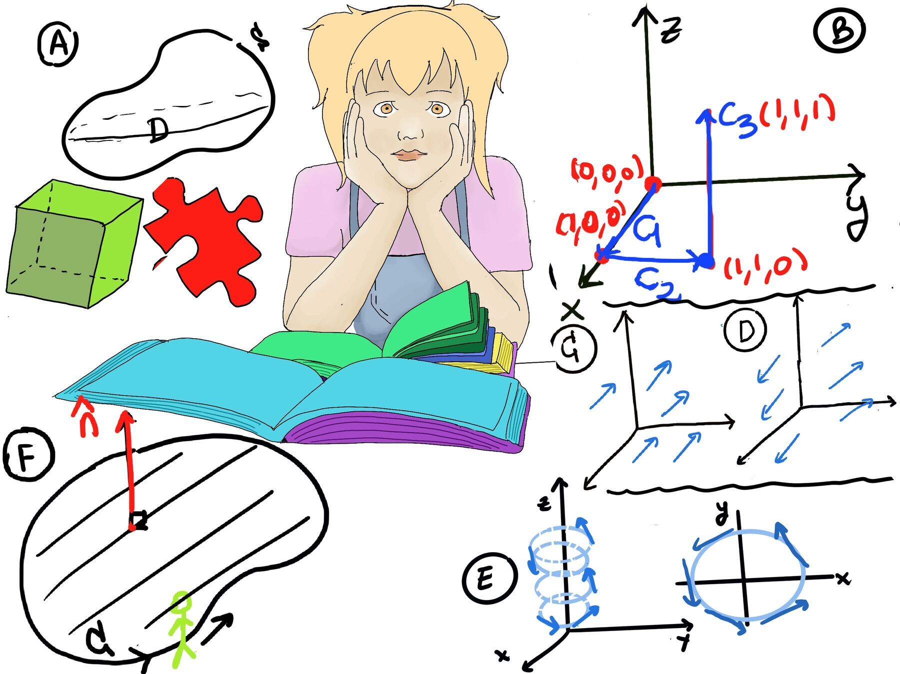
$\int_{C} \vec{F}d\vec{r} = \int_{C} Pdx +Qdy + Rdz = \int_{C} yzdx +xzdy + xydz = \int_{C_1} yzdx +xzdy + xydz + \int_{C_2} yzdx +xzdy + xydz + \int_{C_3} yzdx +xzdy + xydz$

C₁, C₂ live in the xy-plane ⇒ z = 0 ⇒ dz = 0, $\int_{C_1} yzdx +xzdy + xydz + \int_{C_2} yzdx +xzdy + xydz = 0$

C₃: x =1, y = 1 (both are constants) ⇒ dx = dy = 0 ⇒$\int_{C_3} yzdx +xzdy + xydz = \int_{C_3}xydz = \int_{0}^{1} dz = 1$ ⇒ $\int_{C} \vec{F}d\vec{r} = 1$.

In fact, we get the same result because $\vec{F}$ is conservative because $\vec{F} = ∇(x·y·z) = ⟨yz, xz, xy⟩$ and these were two curves, say C and C’, that went from P₀(0, 0, 0) to P₁(1, 1, 1), hence $\int_{C} \vec{F}d\vec{r} = \int_{C’} \vec{F}d\vec{r}$

⇒[Fundamental Theorem of Calculus for line integrals] $\int_{C} \vec{F}d\vec{r} = \int_{C} ∇f d\vec{r} = f(P_1)-f(P_0) = f(1, 1, 1) - f(0, 0, 0) = 1 - 0 = 1$ where f(x, y, z) = x·y·z.

Test for gradient fields

$\vec{F} = ⟨P, Q, R⟩ =¿? ⟨f_x, f_y, f_z⟩$. If so, then P_y = f_xy = f_yx = Q_x and P_z = f_xz = f_zx = R_x, and Q_z = f_yz = f_zy = R_y

Criterion: $\vec{F} = ⟨P, Q, R⟩$ defined in a simple connected region ↭ Pdx + Qdy + Rdz is an exact differential df ↭ P_y = Q_x, P_z = R_x, and Q_z = R_y.

• Example: Find the field vector $\vec{F} = ⟨P, Q, R⟩$ given a differential form and then determine its potential function.

$\int_{C} \vec{F}d\vec{r} = \int_{C} Pdx +Qdy + Rdz$.

The differential form is Pdx +Qdy + Rdz is axydx +(x² +z³)dy + (byz²-4z³)dz where P = axy, Q = x² +z³, R = byz²-4z³. We need to determine the values a and b such that the form is exact.

To do this, we first check the partial derivatives:

P_y = ax = 2x = Q_x ⇒ a = 2. P_z = 0 = 0 = R_x. Finally, Q_z = 3z² = bz² = R_y ⇒ b = 3 ⇒Thus, the differential form becomes 2xydx + (x²+z³)dy +(3yz² -4z³)dz

Find potential

To find the potential function, we have two approaches:

1. Using the line integral, we integrate $\vec{F}$ along a curve C, $f(x_1, y_1, z_1) = \int_{C} \vec{F}d\vec{r} + constant$ where C would typically be (for easy calculations’ sake) a curve from (0, 0, 0) to (x, y, z) similar to Figure B.

   

2. Using the gradient. We find a function f(x, y, z) such that $\vec{F} = ∇f$.

$\int_{C} \vec{F}d\vec{r} = \int_{C} ∇f d\vec{r} = \int_{C} ⟨\frac{∂f}{∂x},\frac{∂f}{∂y},\frac{∂f}{∂z}⟩ d\vec{r} = \int_{C} f_xdx +f_ydy + f_zdz$ where $\vec{F}$ is the vector field, f is the scalar potential function, ∇f is the gradient of f, $d\vec{r}$ is the differential displacement vector along the curve C, and f_x, f_y and f_z are the partial derivatives of f with respect to x, y, and z respectively.

The second approach involves integrating the partial derivatives of f with respect to each variable:

f_x = 2xy ⇒[$\int f(x)dx$] f = x²y + g(y, z).

f_y = x² + z³ =[f = x²y + g(y, z), $\frac{∂f}{∂y} = $] x² +g_y ⇒ g_y = z³ ⇒ g = yz³ + h(z)

f_z = 3yz² -4z³ =[Considering f = x²y +g = x²y +yz³ + h(z)] 3yz²+h’ ⇒ h’(z) = -4z³ ⇒ h = -z⁴ + c.

f = x²y + g(y, z) = x²y + yz³ + h(z) = x²y + yz³ -z⁴ + c.

Curl in 3D

Let our vector field $\vec{F} = P\hat{\mathbf{i}}+ Q\hat{\mathbf{j}}+R\hat{\mathbf{k}}, curl(\vec{F})=(R_y-Q_z)\hat{\mathbf{i}} + (P_z-R_x)\hat{\mathbf{j}}+(Q_x-P_y)\hat{\mathbf{k}}$

If the vector field $\vec{F}$ is defined in a simply connected region (without holes or topological obstacles in the region), then $\vec{F}$ is conservative (a vector field is said to be conservative if it is the gradient of a scalar function, $\vec{F}= ∇f$ where ∇ is the gradient operator) if and only if its curl equals the zero vector, curl($\vec{F}$) = 0 (gradient theorem ⇒ $\vec{F}$ is conservative if the circulation or line integral of $\vec{F}$ around any closed loop or curve is zero, hence if $\vec{F}$ is conservative, then its curl must be zero for any closed loop in the region).

Recall our previous notation, the operator ∇ = $⟨\frac{∂}{∂x},\frac{∂}{∂y},\frac{∂}{∂z}⟩$ and using this notation ∇f = $⟨\frac{∂f}{∂x},\frac{∂f}{∂y},\frac{∂f}{∂z}⟩$

Similarly, ∇·⟨P, Q, R⟩ = $⟨\frac{∂P}{∂x},\frac{∂Q}{∂y},\frac{∂R}{∂z}⟩ = div \vec{F}$

$∇ x \vec{F} = |\begin{smallmatrix}\hat{\mathbf{i}} & \hat{\mathbf{j}} & \hat{\mathbf{k}}\\ \frac{∂}{∂x} & \frac{∂}{∂y} & \frac{∂}{∂z}\\ P & Q & R\end{smallmatrix}| = (\frac{∂R}{∂y}-\frac{∂Q}{∂z})\hat{\mathbf{i}}-(\frac{∂R}{∂x}-\frac{∂P}{∂z})\hat{\mathbf{j}} + (\frac{∂Q}{∂x}-\frac{∂P}{∂i})\hat{\mathbf{k}} = curl \vec{F}$

Geometrically, the curl measures the rotation component in a velocity field. For example, consider a velocity field $\vec{v}$ in some fluid that induces a rotation around the z-axis at an angular velocity w. The velocity field is given by $\vec{v} = ⟨-wy, wx, 0⟩$.

Computing the curl of $\vec{v}$, $curl \vec{v} = ∇ x \vec{v} = 2w\hat{\mathbf{k}}$. It indicates that the curl captures the rotational aspect of the velocity field with the magnitude 2w representing the strength of this rotation and the direction $\hat{\mathbf{k}}$ (the unit vector along the z-axis) along the z-axis indicating the axis of rotation.

Some examples:

1. A constant field $\vec{F} = ⟨a, b, c⟩$, (Figure C), $curl \vec{F} = 0.$
2. A field $\vec{F} = ⟨x, 0, 0⟩$ (Figure D), $curl \vec{F} = 0$, but $div \vec{F} = 1.$
3. A field $\vec{F} = ⟨-y, x, 0⟩$ (Figure E), $curl \vec{F} = 2\hat{\mathbf{k}}$

Bibliography

1. NPTEL-NOC IITM, Introduction to Galois Theory.
2. Algebra, Second Edition, by Michael Artin.
3. LibreTexts Mathematics, Calculus and Calculus 3e (Apex). Abstract and Geometric Algebra, Abstract Algebra: Theory and Applications (Judson).
4. Field and Galois Theory, by Patrick Morandi. Springer.
5. Michael Penn, and MathMajor.
6. Contemporary Abstract Algebra, Joseph, A. Gallian.
7. YouTube’s Andrew Misseldine: Calculus. College Algebra and Abstract Algebra.
8. MIT OpenCourseWare 18.01 Single Variable Calculus, Fall 2007 and 18.02 Multivariable Calculus, Fall 2007.
9. Calculus Early Transcendentals: Differential & Multi-Variable Calculus for Social Sciences.