It is forbidden to kill; therefore all murderers are punished unless they kill in large numbers and to the sound of trumpets, Voltaire

Recall

Definition. A vector $\vec{AB}$ is a geometric object that has magnitude (or length) and direction. Vectors in an n-dimensional Euclidean space can be represented as coordinates vectors in a Cartesian coordinate system.

Definition. The magnitude or length of the vector $\vec{A}$ is given by $|\vec{A}|~ or~ ||\vec{A}|| = \sqrt{a_1^2+a_2^2+a_3^2}$, e.g., $||< 3, 2, 1 >|| = \sqrt{3^2+2^2+1^2}=\sqrt{14}$, $||< 3, -4, 5 >|| = \sqrt{3^2+(-4)^2+5^2}=\sqrt{50}=5\sqrt{2}$, or $||< 1, 0, 0 >|| = \sqrt{1^2+0^2+0^2}=\sqrt{1}=1$.

The dot or scalar product is a fundamental operation between two vectors. It produces a scalar quantity that represents the projection of one vector onto another. The dot product is defined as follows: $\vec{A}·\vec{B} = \sum a_ib_i = a_1b_1 + a_2b_2 + a_3b_3,$ e.g. $\vec{A}·\vec{B} = \sum a_ib_i = ⟨2, 2, -1⟩·⟨5, -3, 2⟩ = a_1b_1 + a_2b_2 + a_3b_3 = 2·5+2·(-3)+(-1)·2 = 10-6-2 = 2.$

Definition. The cross product, denoted by $\vec{A}x\vec{B}$, is a binary operation on two vectors in three-dimensional space. It is a vector that is perpendicular to both of the input vectors (perpendicular to the parallelogram) and has a magnitude equal to the area of the parallelogram formed by the two input vectors.

The direction of the resulting vector is determined by the right-hand rule: if you curl the fingers of your right hand from $\vec{A}$ to $\vec{B}$ (first finger points $\vec{A}$, second finger points to $\vec{B}$), your thumb points in the direction of $\vec{A} \times \vec{B}$.

Matrices provide an efficient way to solve systems of linear equations,

$(\begin{smallmatrix}2 & 3 & 3\\ 2 & 4 & 4\\ 1 & 1 & 2\end{smallmatrix})(\begin{smallmatrix}x_1\\ x_2\\ x_3\end{smallmatrix}) = (\begin{smallmatrix}u_1\\ u_2\\ u_3\end{smallmatrix})$ ↭ A · X = U$ (more convenient and concise notation) where we do the dot products between the rows of A (a 3 x 3 matrix) and the column vector of X (a 3 x 1 matrix).

Given a square matrix A, an inverse matrix A^-1 exists if and only if A is non-singular, i.e., its determinant is non-zero (det(A)≠ 0). The inverse matrix of A, denoted as A^-1, is a matrix such that when multiplied by A yields the identity matrix, i.e., $A \times A^{-1} = A^{-1} \times A = I$

Solving Systems of Linear Equations

Solving a system of linear equations expressed as AX = B involves finding the matrix X when given matrices A and B.

AX = B ⇒[A should be non-singular, det(A)≠0] A^-1(AX) = A^-1B ⇒[Associativity] (A^-1A)X =[Identity Matrix] A^-1B ⇒ X = A^-1B.

Equations of planes

Recall that a point P = (x, y, z) is in the plane ↭[If $\vec{N}$ is perpendicular to the plane, it’s also perpendicular to any vector that lies in the plane, in particular it is perpendicular to $\vec{P_0P}$] $\vec{P_0P}⊥\vec{N}$ where $\vec{N} = ⟨a, b, c⟩$ is a normal vector (orthogonal or perpendicular) to our plane and P₀ = (x₀, y₀, z₀) is a point on the plane ↭ $\vec{P_0P}·\vec{N}=0↭ ⟨x -x_0, y -y_0, z-z_0⟩·⟨a, b, c⟩ ↭a(x-x_0)+b(y-y_0)+c(z-z_0)=0$ this is called the scalar equation of the plane (Figure vii, Credit: Paul’s Online Notes, MIT OpenCourseWare).

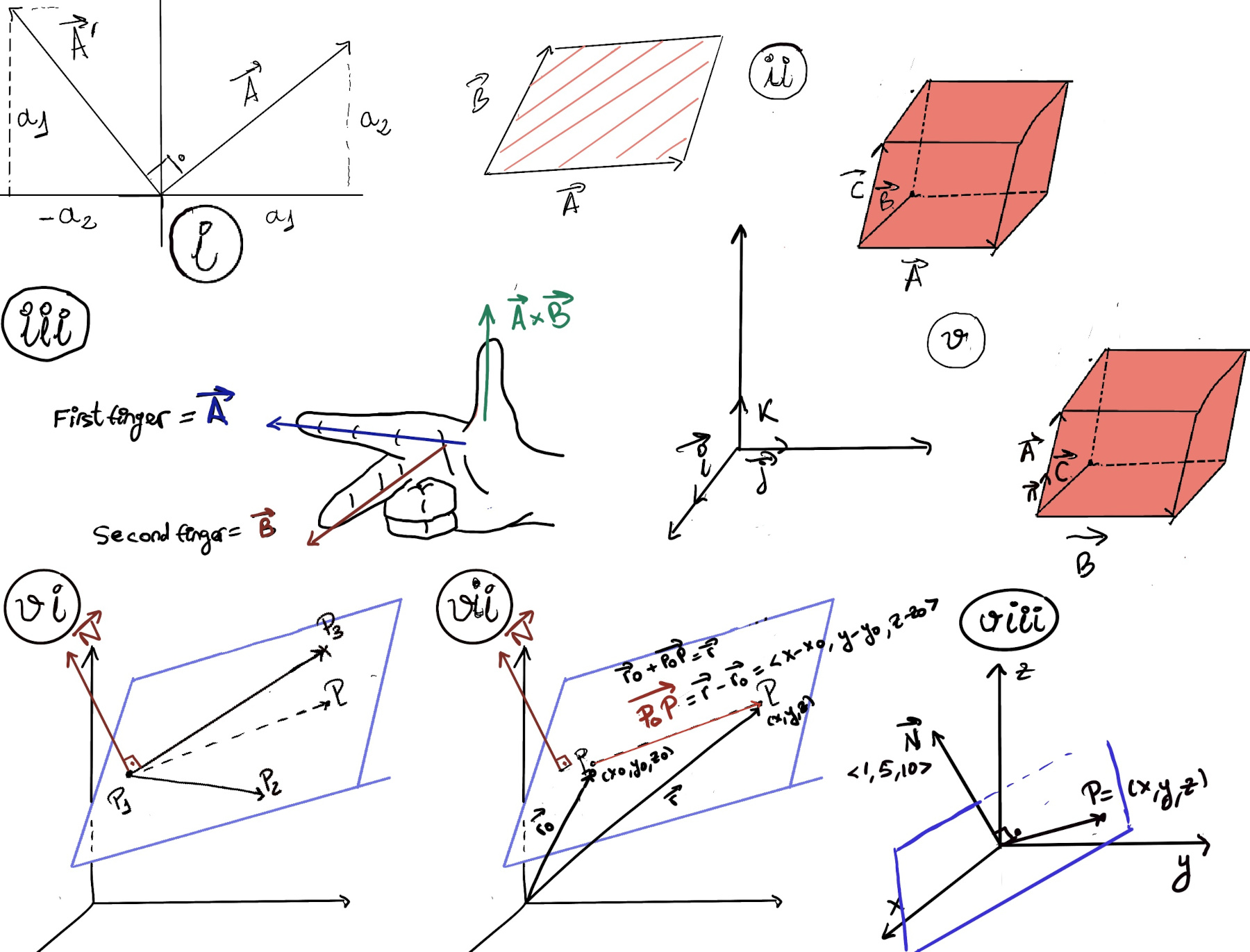
It is often seen as the more familiar ax + by + cz = d where d = ax₀ + by₀ + cz₀, ⟨a, b, c⟩ = $\vec{N}$.

Solved exercises

Find the equation of a plane through the origin with normal vector $\vec{N} = ⟨1, 5, 10⟩$ (Figure viii)

P is in the plane ↭ $\vec{OP}·\vec{N} = 0 ↭ x + 5y +10z = 0.$

Find the equation of a plane through P₀ = (2, 1, -1) with normal vector $\vec{N} = ⟨1, 5, 10⟩$

P is in plane ↭ $\vec{P_0P}·\vec{N}=0↭ ⟨x -x_0, y -y_0, z-z_0⟩·⟨a, b, c⟩ ↭a(x-x_0)+b(y-y_0)+c(z-z_0)=0↭ 1(x-2)+5(y-1)+10(z+1)=0 ↭ x + 5y + 10z = -3$. Notice that if we are given the equation of a plane in this form, we can quickly get our normal vector, namely $\vec{N} = ⟨1, 5, 10⟩$ or alternatively, if know our normal vector, we can write down the left-hand side of the plane’s equation, and we plug in P₀ in the left-hand side to get the value of the right-hand side of the plane’s equation.

Are the vector $\vec{v} = ⟨1, 2, -1⟩$ and the plane x + y + 3z = 5 parallel, perpendicular, or neither?

We have the scalar equation of the plane ⇒ $\vec{N} = ⟨1, 1, 3⟩$

$\vec{v}·\vec{N} = 1·1 + 2·1 + (-1)3 = 1 + 2 -3 = 0$ ⇒ $\vec{v}$ and $\vec{N}$ are perpendicular to each other ⇒ $\vec{v}$ is parallel to the plane.

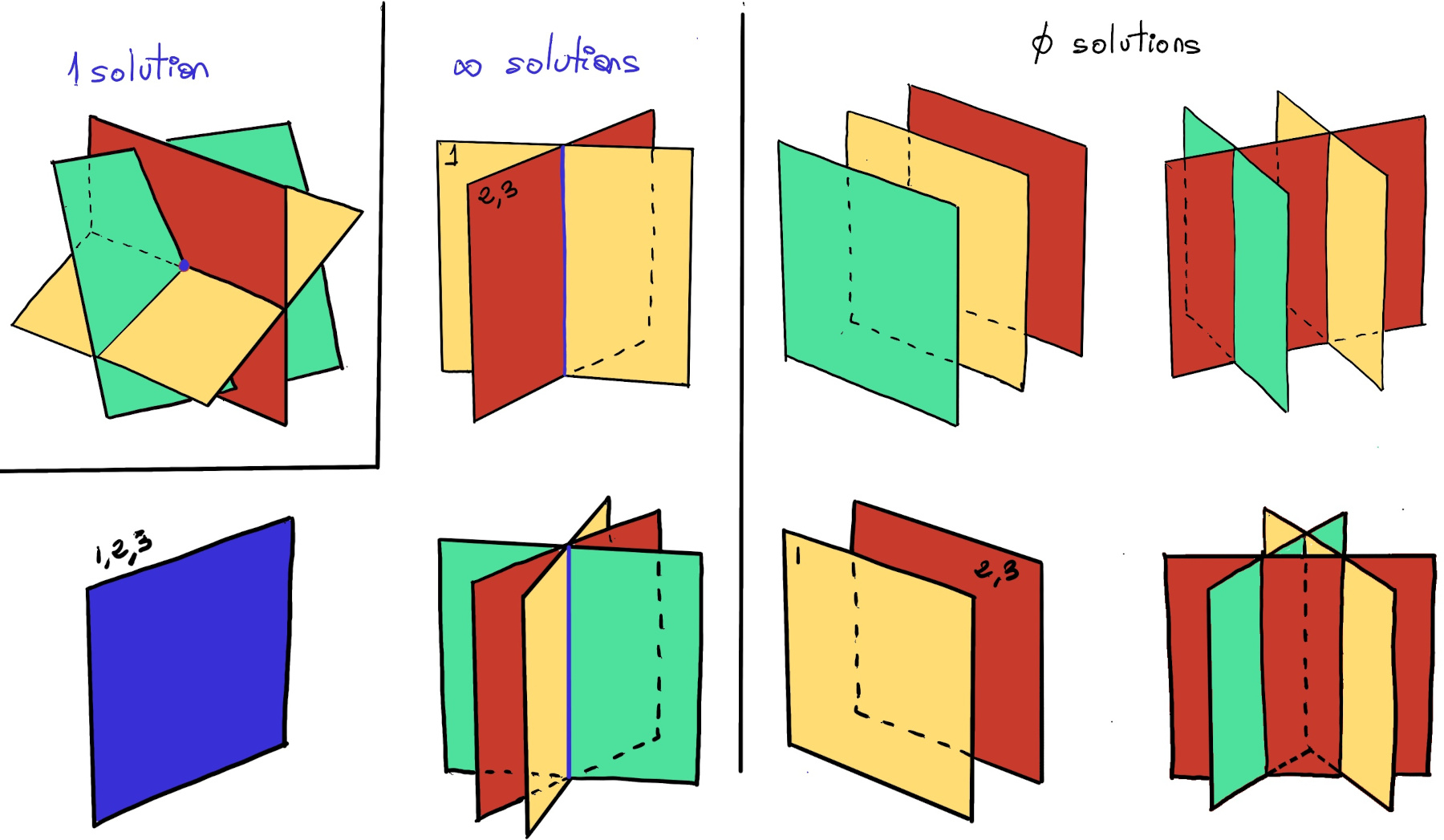
Solving Systems of Linear Equations

A system of three equations with three unknowns represents three planes in three dimensional space. When solving the system, you are figuring out how the planes intersect.

The solution to AX = B is given by X = A^-1B, but it is not always the case. A system of three linear equations in three variables can either have no solution, one solution (a point of intersection of the three planes), or infinitely many solutions (a line or plane in three-dimensional space, the equations are dependent).

Let R be a commutative ring with unity. Let A ∈ R^n×n be a square matrix of order n. A is invertible if and only if its determinant is invertible in R. If R = ℚ, ℝ or ℂ, A is invertible if and only if its determinant is non-zero.

$\begin{cases} x + z = 1 \\ x + y = 2 \\ x + 2y +3z = 3 \end{cases}$

From the first equation, we can express x in terms of z: x = 1 -z.
Substituting x = 1 - z into the second equation, we get: 1 -z + y = 2, and solving this equation for y, we get: y = 1 + z.
Now, we have expressions for x and y in terms of z. Substituting these into the third equation: 1 -z +2(1 + z) + 3z = 3 ↭ 1 -z + 2 +2z +3z = 3 ↭ 3 + 4z = 3 ↭ z = 0 ⇒ x = 1 and y = 1. Therefore, the solution is the point (1, 1, 0).

A homogeneous system of linear equations is one in which all of the constant terms are zero. A homogeneous system always has at least one solution (all there planes pass through the origin, hence the origin is always a solution), namely the zero vector.

An n×n homogeneous system of linear equations has a unique solution (the trivial solution) if and only if its determinant is non-zero ⇒ AX = 0 ↭ X = A^-1·0 = 0. If this determinant is zero, then the system has an infinite number of solutions.

$\begin{cases} x + z = 0 \\ x + y = 0 \\ x + 2y +3z = 0 \end{cases}$

(0, 0, 0) is a trivial solution.

In the General case, if Ax = b and det(A) ≠ 0, then A^-1 exists, so x = A^-1b is the unique solution of the system. If det(A) = 0, then the system of equation either has infinitely many solutions, or no solutions.

Solved exercise

Let A = $(\begin{smallmatrix}1 & 3 & 2\\ 2 & 0 & -1\\ 1 & 1 & 0\end{smallmatrix})$, det(A) = 2, and A^-1 = $\frac{1}{2}(\begin{smallmatrix}1 & ? & ?\\ -1 & -2 & 5\\ 2 & 2 & -6\end{smallmatrix})$, compute A^-1 in an efficient way.

We don’t need to calculate the Minors completely, Minors = $(\begin{smallmatrix}x & x & x\\ -2 & x & x\\ -3 & x & x\end{smallmatrix})$ ⇒ Cofactors = $(\begin{smallmatrix}x & x & x\\ 2 & x & x\\ -3 & x & x\end{smallmatrix})$ ⇒ Transpose = $(\begin{smallmatrix}x & 2 & -3\\ x & x & x\\ x & x & x\end{smallmatrix})$ ⇒[Dividing by det(A)=2] A^-1 = $\frac{1}{2}(\begin{smallmatrix}1 & 2 & -3\\ -1 & -2 & 5\\ 2 & 2 & -6\end{smallmatrix})$.

Solve the system of equation,

$\begin{cases} x + 3y + 2z = 1 \\ 2x -z = -2 \\ x +y = 1 \end{cases}$

To solve the system of equations using matrices, we can represent the system in matrix form AX = B, where: A = $(\begin{smallmatrix}1 & 3 & 2\\ 2 & 0 & -1\\ 1 & 1 & 0\end{smallmatrix})$ and B = $(\begin{smallmatrix}1\\ -2\\ 1\end{smallmatrix})$ ⇒ X = A^-1·B =[Previous exercise] $\frac{1}{2}(\begin{smallmatrix}1 & 2 & -3\\ -1 & -2 & 5\\ 2 & 2 & -6\end{smallmatrix})·(\begin{smallmatrix}1\\ -2\\ 1\end{smallmatrix}) = \frac{1}{2}(\begin{smallmatrix}-6\\ 8\\ -8\end{smallmatrix})=(\begin{smallmatrix}-3\\ 4\\ -4\end{smallmatrix})$. Therefore, the solution to the system of equations is x = −3, y = 4, and z = −4.

Find the value of c where the matrix M is not invertible where M = $(\begin{smallmatrix}1 & 3 & c\\ 2 & 0 & -1\\ 1 & 1 & 0\end{smallmatrix})$

Recall that a matrix is not invertible if its determinant is zero, indicating that its columns are not linearly independent.

$\left| M \right| = a_{11}(a_{22}a_{33} - a_{23}a_{32}) - a_{12}(a_{21}a_{33} - a_{23}a_{31}) + a_{13}(a_{21}a_{32} - a_{22}a_{31})$ where a_ij represents the element in the ith row and jth column of matrix M.

det(M) = 1(0⋅0−1⋅1)−3(2⋅0−1⋅1)+c(2⋅1−1⋅0) = 1(−1)−3(−1)+c(2) = 2 + 2c = 0 ⇒ c = 1.

Solve the system of equations MX = 0, that is, M = $(\begin{smallmatrix}1 & 3 & 1\\ 2 & 0 & -1\\ 1 & 1 & 0\end{smallmatrix})$,

$\begin{cases} x + 3y + z = 0 \\ 2x -z = 0 \\ x +y = 0 \end{cases}$

The obvious solution is (0, 0, 0).

If we multiply the third equation by 3, 3x + 3y = 0 and subtract it to the second equation 2x -z = 0, we get x + 3y +z = 0, that is, the first equation ⇒ If one of the equations can be expressed as a linear combination of the others ⇒ it results in the system having infinitely many solutions.

Another way of putting this is as follows, our system of equations can be expressed as follows, ⟨x, y, z⟩·⟨1, 3, 1⟩ = 0, ⟨x, y, z⟩·⟨2, 0, -1⟩ = 0, ⟨x, y, z⟩·⟨1, 1, 0⟩ = 0,

Recall, if the dot product between a pair of vectors is zero, then the two vectors are orthogonal. Thus we see that if X is in the null space of M (The null space of a matrix M is the set of all solutions to the homogeneous equation M·X = 0), it has to be orthogonal to every row-vector of M.

As we already know, the cross product of two non-collinear vectors gives a vector perpendicular to the plane determined by the vectors, and therefore, to find the solution ⟨x, y, z⟩, we take the cross product of ⟨1, 3, 1⟩ and ⟨2, 0, -1⟩.

v = $(\begin{smallmatrix}\vec{i} & \vec{j} & \vec{k}\\ 1 & 3 & 1\\ 2 & 0 & 1\end{smallmatrix})$ = ⟨-3, 3, -6⟩. Specifically, any scalar multiple of this vector is also a solution to the system. The line of solution (it passes through (0, 0, 0) and contains the vector $\vec{N}= ⟨-3, 3, -6⟩$) has parametric solutions x = -3t, y = 3t, z = -6t.

Bibliography

This content is licensed under a Creative Commons Attribution-NonCommercial-ShareAlike 4.0 International License and is based on MIT OpenCourseWare [18.01 Single Variable Calculus, Fall 2007].

NPTEL-NOC IITM, Introduction to Galois Theory.
Algebra, Second Edition, by Michael Artin.
LibreTexts, Calculus and Calculus 3e (Apex). Abstract and Geometric Algebra, Abstract Algebra: Theory and Applications (Judson).
Field and Galois Theory, by Patrick Morandi. Springer.
Michael Penn, and MathMajor.
Contemporary Abstract Algebra, Joseph, A. Gallian.
YouTube’s Andrew Misseldine: Calculus. College Algebra and Abstract Algebra.
MIT OpenCourseWare 18.01 Single Variable Calculus, Fall 2007 and 18.02 Multivariable Calculus, Fall 2007.
Calculus Early Transcendentals: Differential & Multi-Variable Calculus for Social Sciences.