Second derivative test

Second derivative test

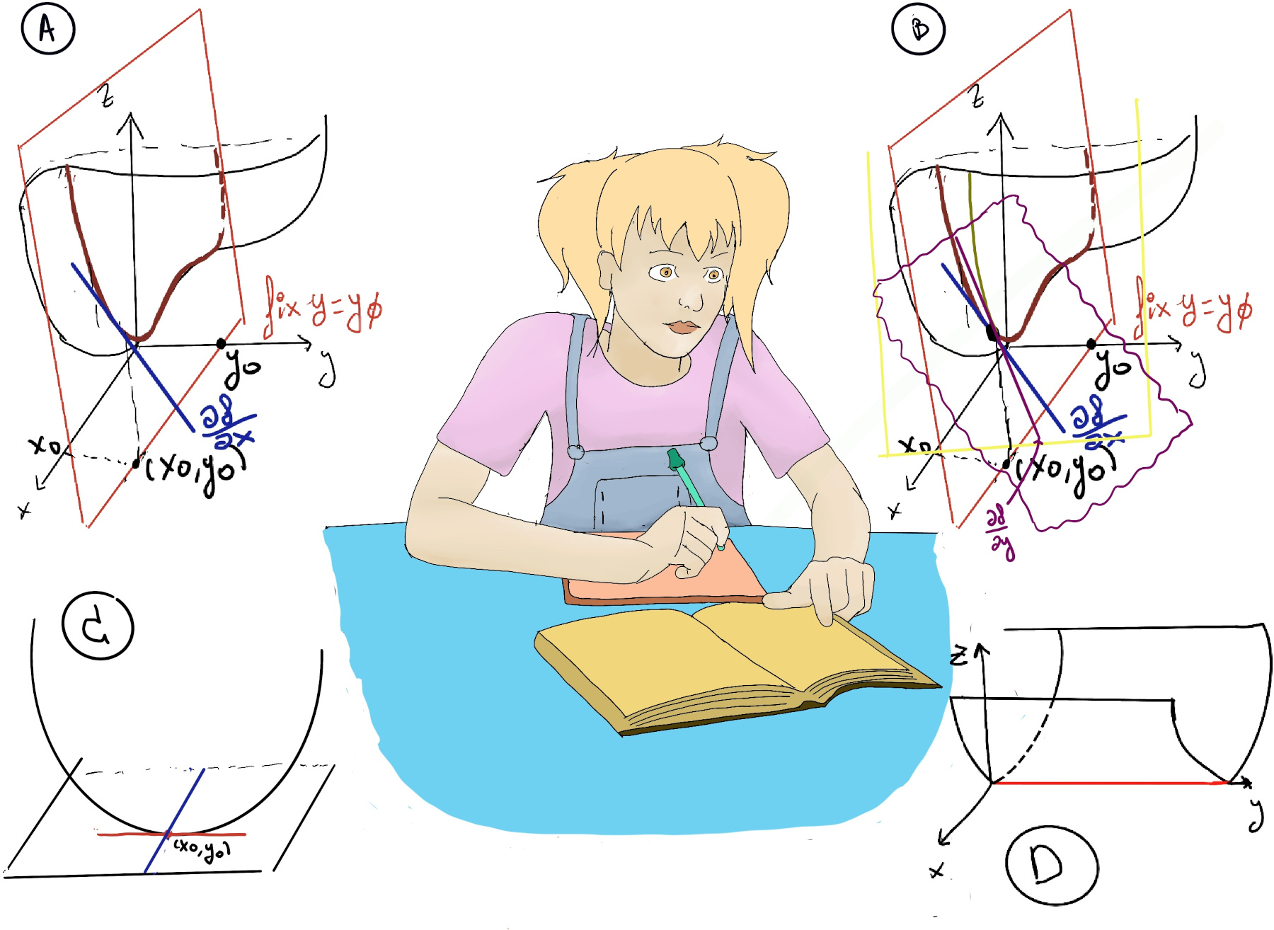
Let’s consider w = ax² + bxy + cy², e.g., w = x² +2xy + 3xy² = (x+y)² + 2y², and obviously the origin is a minimum.

In general, w = $a(x^2+\frac{b}{a}xy) +cy^2$ =[Consider that $a(x^2+\frac{b}{2a}xy)^2 = ax^2 +a2x\frac{b}{2a}y + a\frac{b^2}{4a^2}y^2$] $a(x+\frac{b}{2a}y)^2+(c-\frac{b^2}{4a})y^2 = \frac{1}{4a}[4a^2(x+\frac{b}{2a}y)^2+(4ac-b^2)y^2]$

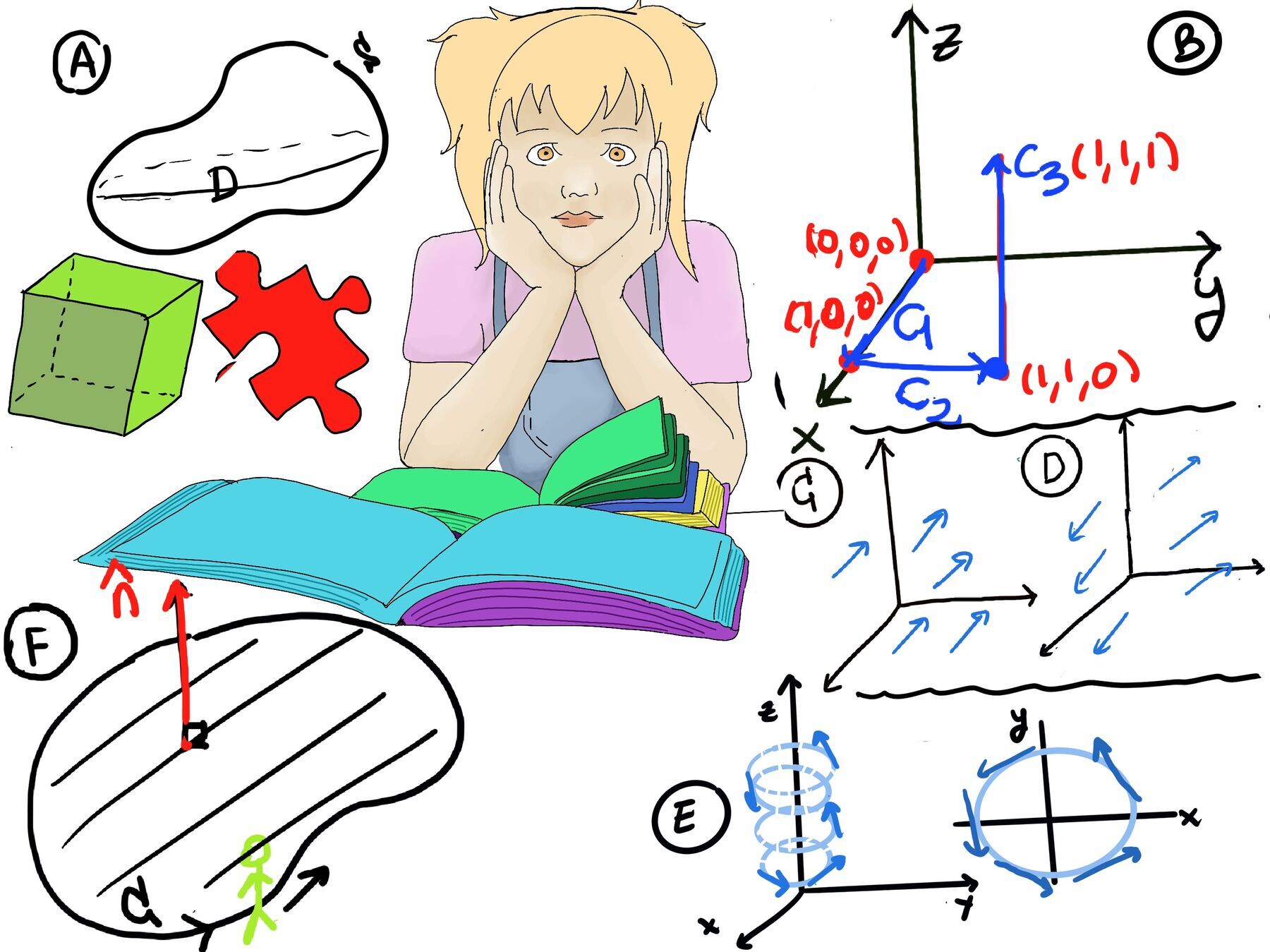
If 4ac -b² = 0 ⇒ w = $a(x+\frac{b}{2a}y)^2$, e.g., w = x², there is a degenerate critical point (minimum or maximum depending on the sign of a), it is basically a valley which bottom is completely flat, Figure D, hence there are critical points along the y-axis. If 4ac -b² ≥ 0 ⇒$4a^2(x+\frac{b}{2a}y)^2+(4ac-b^2)y^2 ≥ 0$, then there are two cases:

1. If a > 0, then we have a minimum.
2. If a < 0, then we have a maximum.

Notice that w = ax² + bxy + cy² = $y^2[a(\frac{x}{y})^2+b(\frac{x}{y})+c]$. If b² -4ac > 0 (we can reformulate $a(\frac{x}{y})^2+b(\frac{x}{y})+c$ as at² +bt +c), w takes positive and negative values, so there is a saddle point.

If b² -4ac < 0 ⇒ $a(\frac{x}{y})^2+b(\frac{x}{y})+c$ is always positive or negative depending on the sign of a, and we will get a minimum or a maximum.

In multivariable calculus, the second derivative test is a method used to determine the nature of critical points of a function of two variables. It helps in determining whether a critical point is a local maximum, local minimum, or a saddle point.

We calculate the second partial derivatives of the function with respect to both variables x and y, i.e., $\frac{\partial^2 f}{\partial x^2} = f_{xx} = A, \frac{\partial^2 f}{\partial y^2} = f_{yy} = C, f_{xy} = \frac{\partial^2 f}{\partial x \partial y}= \frac{\partial^2 f}{\partial y \partial x} = f_{yx} = B$ (this is left to the reader to demonstrate).

There are four cases: (D = f_xx·f_yy-(f_xy)²= AC -B²)

1. If D > 0 and f_xx > 0, then the critical point is a local minimum.
2. If D > 0 and f_xx < 0, then the critical point is a local minimum.
3. If D < 0, then the critical point is a local minimum.
4. If D = 0, the test is inconclusive.

Going back to our previous examples, w = ax² + bxy + cy², $\frac{\partial^2 f}{\partial x^2} = 2a, \frac{\partial^2 f}{\partial x \partial y} = b, \frac{\partial^2 f}{\partial y^2} =2c$, D = f_xx·f_yy-(f_xy)² = 4ac -b²

Observe that the quadratic approximation $\Delta f ≈ f_x (x -x_0) + f_y(y - y_0) + \frac{1}{2}f_{xx}(x-x_0)^2+ f_{xy}(x-x_0)(y-y_0) + \frac{1}{2}f_{yy}(y-y_0)^2$ =[Critical points ] $\frac{1}{2}f_{xx}(x-x_0)^2+ f_{xy}(x-x_0)(y-y_0) + \frac{1}{2}f_{yy}(y-y_0)^2$, hence the general case reduces to the quadratic case where $\frac{1}{2}f_{xx} = \frac{1}{2}A = a, f_{xy} = B = b, \frac{1}{2}f_{yy} = \frac{1}{2}C = c$

The reason why this argument does not work is that our quadratic approximation only works when the higher order terms (derivatives) are not very significant. In the degenerate case, this is not the case.

• Example: f(x, y) = x + y + ¹⁄_xy where x, y > 0.

First, we need to calculate the critical points, $f_x =1-\frac{1}{x^2y} = 0, f_y =1-\frac{1}{xy^2} = 0↭ x^2y = 1~ (i), xy^2 = 1~ (ii)$. Let compute (i)/(ii) x = y ⇒ y³ = 1 ⇒[y > 0] y = 1 ⇒[x = y] x = 1. Hence, there is only one critical point (1, 1).

Let’s compute the second partial derivatives, $f_{xx}=\frac{2}{x^3y}$ ⇒ A = 2, $f_{xy}=\frac{1}{x^2y^2}$ ⇒ B = 1, and $f_{yy}=\frac{2}{xy^3}$ ⇒ C = 2 ⇒ D = AC -B² = 2·2 -1² = 3 > 0, and A = f_xx > 0 ⇒ local minimum.

The maximum is achieved when f → ∞ ↭ x → ∞ or y → ∞ or x, y → 0, and it is not a critical point, so in general we need to check both the critical points and the boundaries to know what happens.

Bibliography

1. NPTEL-NOC IITM, Introduction to Galois Theory.
2. Algebra, Second Edition, by Michael Artin.
3. LibreTexts, Calculus and Calculus 3e (Apex). Abstract and Geometric Algebra, Abstract Algebra: Theory and Applications (Judson).
4. Field and Galois Theory, by Patrick Morandi. Springer.
5. Michael Penn, and MathMajor.
6. Contemporary Abstract Algebra, Joseph, A. Gallian.
7. YouTube’s Andrew Misseldine: Calculus. College Algebra and Abstract Algebra.
8. MIT OpenCourseWare 18.01 Single Variable Calculus, Fall 2007 and 18.02 Multivariable Calculus, Fall 2007.
9. Calculus Early Transcendentals: Differential & Multi-Variable Calculus for Social Sciences.