Partial derivatives

Partial derivatives

Partial derivatives are derivatives of a function of multiple variables, say f(x₁, x₂, ···, x_n) with respect to one of those variables, with the other variables held constant. They measure how the function changes as one variable changes, while keeping the others constant.

$\frac{\partial f}{\partial x}(x_0, y_0) = \lim_{\Delta x \to 0} \frac{f(x_0+\Delta x, y_0)-f(x_0, y_0)}{\Delta x}$

Similarly, $\frac{\partial f}{\partial y}(x_0, y_0) = \lim_{\Delta y \to 0} \frac{f(x_0, y_0+\Delta y)-f(x_0, y_0)}{\Delta y}$

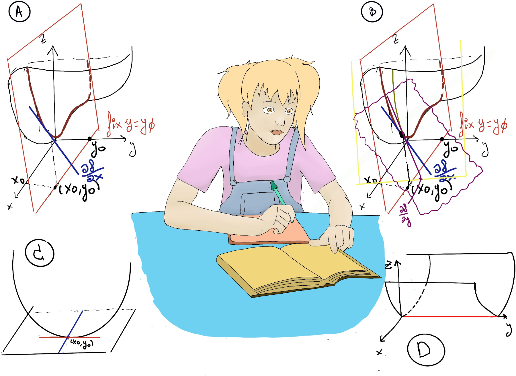
Geometrically, the partial derivative $\frac{\partial f}{\partial x}(x_0, y_0)$ at a point (x₀, y₀) can be interpreted as the slope of the tangent line to the curve formed by the intersection of the surface defined by f(x,y) and the plane y = y₀. Similarly, $\frac{\partial f}{\partial x}(x_0, y_0)$ represents the slope of the tangent line to the curve formed by the intersection of the surface defined by f(x,y) and the plane x = x₀ (Figure A).

Example. Let f(x, y) = x³y + y², $\frac{\partial f}{\partial x} = f_x = 3x^2·y, \frac{\partial f}{\partial y} = f_y = x^3+2y.$

The linear approximation formula for a function f(x,y) around the point (x₀, y₀) ≈ $f(x_0, y_0) + \frac{\partial f}{\partial x}(x_0, y_0)(x -x_0)+ \frac{\partial f}{\partial y}(x_0, y_0)(y -y_0)$.

The partial derivatives of the function with respect to x and y evaluated at the point (x₀, y₀) represent the rates of change of the function in the x- and y-directions at that point. This formula represents the equation of the tangent plane to the surface defined by the function f(x,y) at the point (x₀, y₀) where $Δz ≈ \frac{\partial f}{\partial x}(x_0, y_0)(x -x_0)+ \frac{\partial f}{\partial y}(x_0, y_0)(y -y_0)$ (Figure B).

Let’s suppose that $\frac{\partial f}{\partial x}(x_0, y_0) = a$, then L₁ = z = z₀+ a(x -x₀) where y =[constant] y₀ and $\frac{\partial f}{\partial y}(x_0, y_0) = b$, then L₂ = z = z₀+ b(y -y₀) where x =[constant] x₀. Therefore, L₁ and L₂ are both tangent to the graph z = f(x, y) and together determine a plane given by the formula z = z₀ + a(x -x₀) + b(y - y₀), and this approximation states that the graph of f is close to its tangent plane in the intermediate vicinity of the point (x₀, y₀). ​

Approximation problems

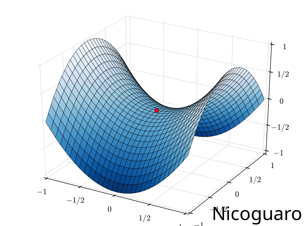
At a local minimum or maximum of a function f(x,y), the partial derivatives with respect to each variable are zero: $\frac{\partial f}{\partial x}(x_0, y_0) = 0, \frac{\partial f}{\partial y}(x_0, y_0) = 0$, that is, the horizontal plane to the graph z = f(x, y) is horizontal (Figure C). However, it’s essential to understand that this condition is necessary but not a sufficient condition for a point to be a local minimum or maximum.

Critical points in multivariable functions can indeed be local minimums, local maximums, saddle points (where the slopes (derivatives) in orthogonal directions are all zero (a critical point), but which is not a local extremum of the function, e.g., a relative minimum along one axial direction and at a relative maximum along the crossing axis, f(x, y) = x² + y² has a critical point at (0, 0) that is a saddle point), or points of inflection.

Formally, let f(x₁, x₂, ···, x_n) be a function of n variables. A point (x₁, x₂, ···, x_n) in the domain of f is considered a critical point if the gradient of f at that point is the zero vector or if the gradient does not exist. In particular, n = 2, $\frac{\partial f}{\partial x}(x_0, y_0) = 0$ and $\frac{\partial f}{\partial y}(x_0, y_0) = 0$

Example: f(x, y) = x² -2xy +3y² + 2x -2y, $\frac{\partial f}{\partial x} = 2x -2y +2, \frac{\partial f}{\partial y} = -2x +6y -2$

$\begin{cases} x -2y +2 = 0 \\ -2x +6y -2 = 0 \end{cases}$ ⇒[By adding them] 4y = 0 ⇒y = 0 ⇒ -2x + 2 = 0 ⇒ x = -1 ⇒ Critical point (-1, 0)

Least Squares Interpolation

Least squares interpolation is a method used to fit a curve to a set of data points in such a way that the sum of the squares of the differences between the observed and predicted values is minimized (we try to minimize the total square error).

As a introductory example, let’s suppose that we have a set of data point (x_i, y_i) and choose a linear model (y = ax +b) to represent the relationship between the independent and dependent variables, i.e., the deviation for each data point equals y_i -(ax_i +b). Therefore, our goal is to minimize D(a, b) = $\sum_{i=1}^n [y_i-(ax_i +b)]^2$

$\frac{\partial D}{\partial a} = \sum_{i=1}^n 2(y_i-(ax_i +b))(-x_i)=0, \frac{\partial D}{\partial b} = \sum_{i=1}^n 2(y_i-(ax_i +b))(-1)=0$

$\begin{cases} \sum_{i=1}^n (x_i^2a+x_ib-x_iy_i)= 0 \\ \sum_{i=1}^n (x_ia +b -y_i)=0 \end{cases}$

$\begin{cases} (\sum_{i=1}^n x_i^2)a + (\sum_{i=1}^nx_i)b = \sum_{i=1}^n x_iy_i \\ (\sum_{i=1}^n x_i)a + nb = \sum_{i=1}^n y_i \end{cases}$

This is a 2 x 2 linear system and we need to solve it for a and b.

Moore’s Law

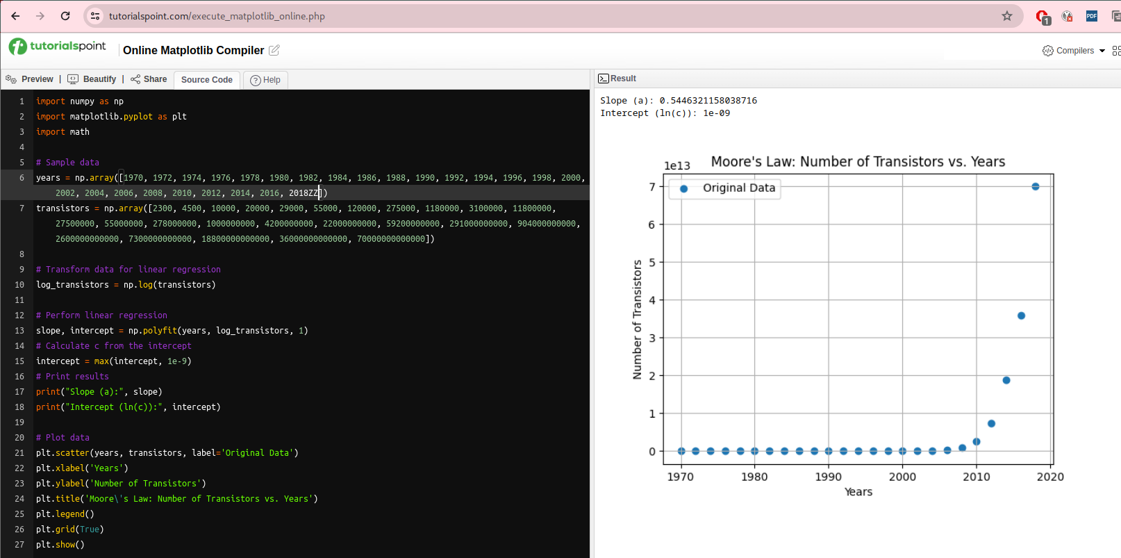
Moore’s law is the observation that the number of transistors in an integrated circuit (IC) doubles approximately every two years. Consider the exponential function: y = $c·e^{ax}$ where y represents the number of transistors on an integrated circuit; c is a constant multiplier that accounts for initial conditions; a is the growth rate parameter; and x time measured in years.

When we examine the doubling of transistors every two years, it aligns with the exponential function’s behavior. However, y = $c·e^{ax} ↭ ln(y) = ln(c) + ln(e^{ax}) ↭ ln(y) = ln(c) + ax$, and that is the linear best fit. Let’s search for the best straight line fit for the log(y) where the most important lines are:

import numpy as np
import matplotlib.pyplot as plt
import math

# Sample data
years = np.array([1970, 1972, 1974, 1976, 1978, 1980, 1982, 1984, 1986, 1988, 1990, 1992, 1994, 1996, 1998, 2000, 2002, 2004, 2006, 2008, 2010, 2012, 2014, 2016, 2018ZZ])
transistors = np.array([2300, 4500, 10000, 20000, 29000, 55000, 120000, 275000, 1180000, 3100000, 11800000, 27500000, 55000000, 278000000, 1000000000, 4200000000, 22000000000, 59200000000, 291000000000, 904000000000, 2600000000000, 7300000000000, 18800000000000, 36000000000000, 70000000000000])

# Transform data for linear regression
log_transistors = np.log(transistors)

# Perform linear regression (Least squares polynomial fit)
slope, intercept = np.polyfit(years, log_transistors, 1)

Bibliography

1. NPTEL-NOC IITM, Introduction to Galois Theory.
2. Algebra, Second Edition, by Michael Artin.
3. LibreTexts, Calculus and Calculus 3e (Apex). Abstract and Geometric Algebra, Abstract Algebra: Theory and Applications (Judson).
4. Field and Galois Theory, by Patrick Morandi. Springer.
5. Michael Penn, and MathMajor.
6. Contemporary Abstract Algebra, Joseph, A. Gallian.
7. YouTube’s Andrew Misseldine: Calculus. College Algebra and Abstract Algebra.
8. MIT OpenCourseWare 18.01 Single Variable Calculus, Fall 2007 and 18.02 Multivariable Calculus, Fall 2007.
9. Calculus Early Transcendentals: Differential & Multi-Variable Calculus for Social Sciences.