Lagrange Multipliers

All warfare is based on deception, Sun tzu, The Art of War.

Lagrange Multipliers

It is a strategy for finding the local maxima and minima of a function, say f(x, y, z), subject to a equality constraint, g(x, y, z) = c. It uses the fact that any point where f(x, y, z) has a constraint extremum (maximum or minimum), the gradient of f is parallel to the gradient of g. Formally, this can be represented as ∇f = λ∇g where λ is the Lagrange multiplier.

Let’s propose an example problem. Let’s calculate the point closet to the origin on the hyperpola xy = 3.

We can set up the problem as follows: we want to minimize the function f(x, y) = $\sqrt{x^2+y^2}$ subject to the constraint g(x, y) = xy = 3, it is like finding the highest or lowest point on a mountain or hill subject to the fact you can only walk along a trail. We will simplify the problem by getting rid of the square, so we will try to minimize f(x, y) = x^2 + y^2 (Figure C and D).

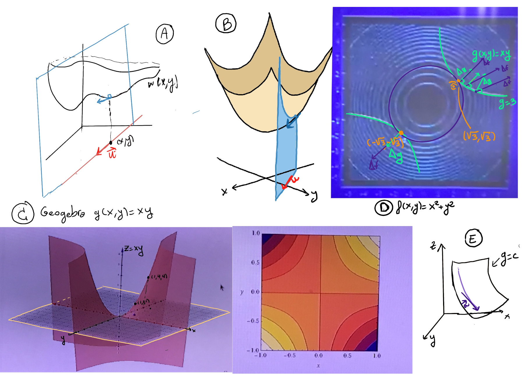
At the minimum, the level curve of f is tangent to the parabola g. In general, lagrange multipliers is about finding (x, y) where the level curves of f and g are tangent to each other, and this is due to the fact that gradients are tangents to contour lines, hence the gradient of f is parallel to the gradient of f, that is, proportional to each other ↭ ∇f = λ∇g where λ is the Lagrange multiplier.

The gradient of a function at $\vec{a}$ represents the direction in which f increases at the greatest rate so, if one writes down a contour diagram with each contour representing a level set of f (levels of equal value), ∇f($\vec{a}$) represents the direction from $\vec{a}$ in which the contours are least sparse.

When we talk about finding a minimum or maximum of a function f(x, y, z) subject to a constraint g(x, y, z) = c, we are essentially looking for points where f does not increase or decrease when moving along the level curve (or surface) defined by g(x, y, z) = c. Then, the constraint g(x, y, z) = c, defines a level curve in two dimensions or a lever surface, so the rate of change of f in any direction $\vec{a}$ that is tangent to the level curve g = c must be zero at a constraint extremum because if it weren’t, you could move slightly in the direction of increase (for a maximum) or decrease (for a minimum) while still staying on the level curve or surface g = c, indicating that the current point is not actually an extremum, i.e., $\frac{df}{ds}\bigg|_{\vec{a}} = 0$ (Figure E)

$\frac{df}{ds}\bigg|_{\vec{a}} = ∇f·\vec{a} = 0$ ⇒ $\vec{a} ⊥ ∇f$ ⇒ ∇f ⊥ level set of g = c and we know that ∇g ⊥ level set of g = c ⇒ ∇f || ∇g.

Therefore, our problem is reformulated as a system of equations,

$\begin{cases} \frac{∂f}{∂x} = λ\frac{∂g}{∂x} \\ \frac{∂f}{∂y} = λ\frac{∂g}{∂y} \\ g = c \end{cases}$

This yields critical points that need to be evaluated to determine if they are maxima, minima, or saddle points, taking into account the constraint g = c. The method does not tell whether a critical point is a minimum, maximum, or saddle point.

$\begin{cases} f_x = λg_x \\ f_y = λg_y \\ g = c\end{cases}$

In our particular example, f(x, y) = x^2 + y^2, g = xy,

$\begin{cases} 2x = λy \\ 2y = λx \\ xy = 3\end{cases}$

$\begin{cases} 2x - λy = 0 \\ λx -2y = 0 \\ xy = 3\end{cases}$

$(\begin{smallmatrix}2 & -λ\\ λ & -2\end{smallmatrix})(\begin{smallmatrix}x\\ y\end{smallmatrix}) = (\begin{smallmatrix}0\\ 0\end{smallmatrix})$.

The trivial solution (0, 0) does not satisfy the constraint (0·0 ≠ 3). We have other solutions if det(M) = 0 ↭ $|\begin{smallmatrix}2 & -λ\\ λ & -2\end{smallmatrix}|=-4+λ^2=0 ↭ λ^2 = 4 ↭ λ = ± 2$

1. If λ = 2 ⇒ x = y, x² = 3 ⇒ There are two solutions: $\sqrt{3},\sqrt{3}$ or $-\sqrt{3},-\sqrt{3}$
2. If λ = -2, x = -y, -x² = 3 ⇒ There are no solutions.

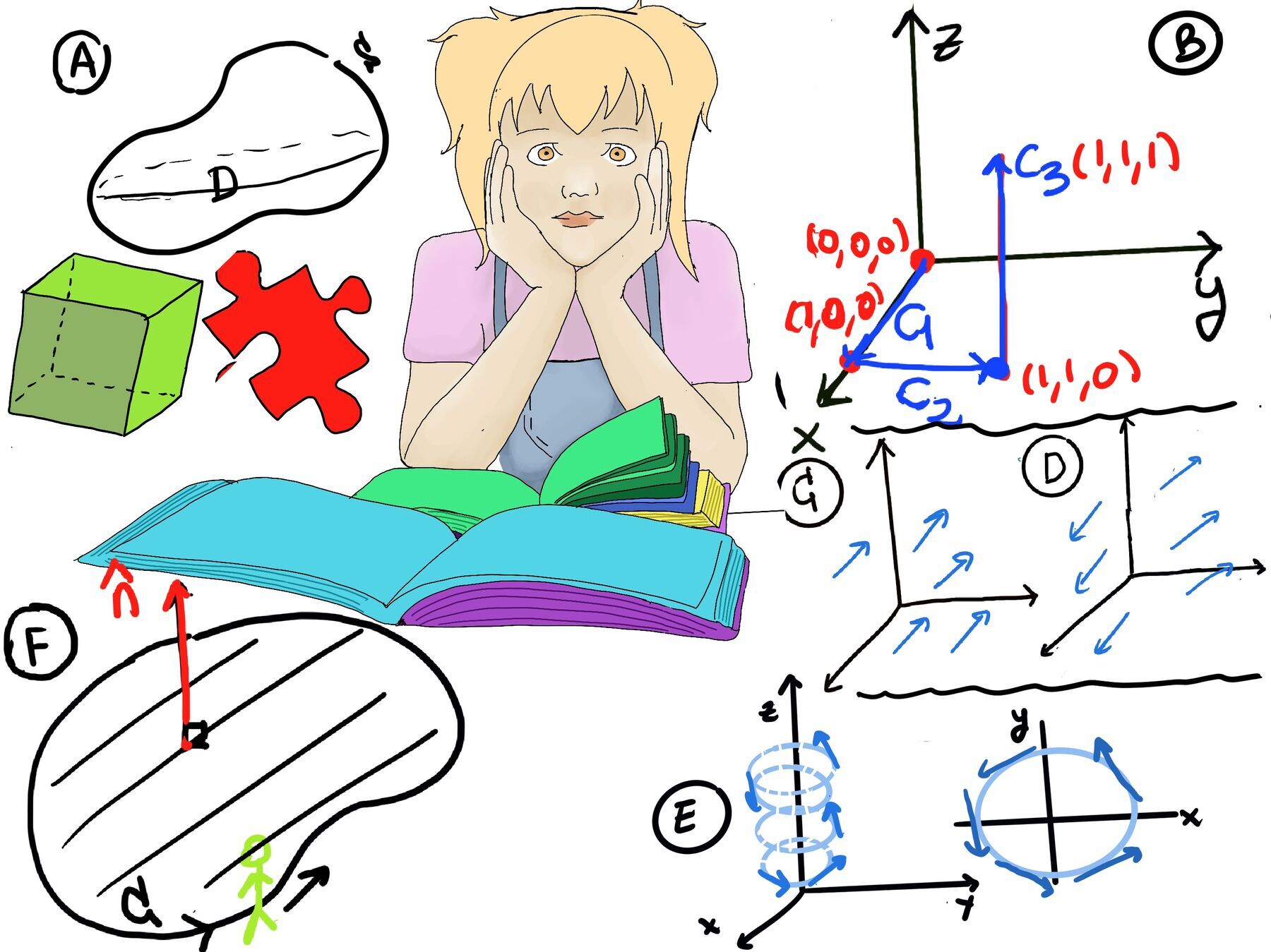
Suppose that we want to build a pyramid with a given triangular base and a given volume and we want to minimize the total surface area (Figure i, ii)

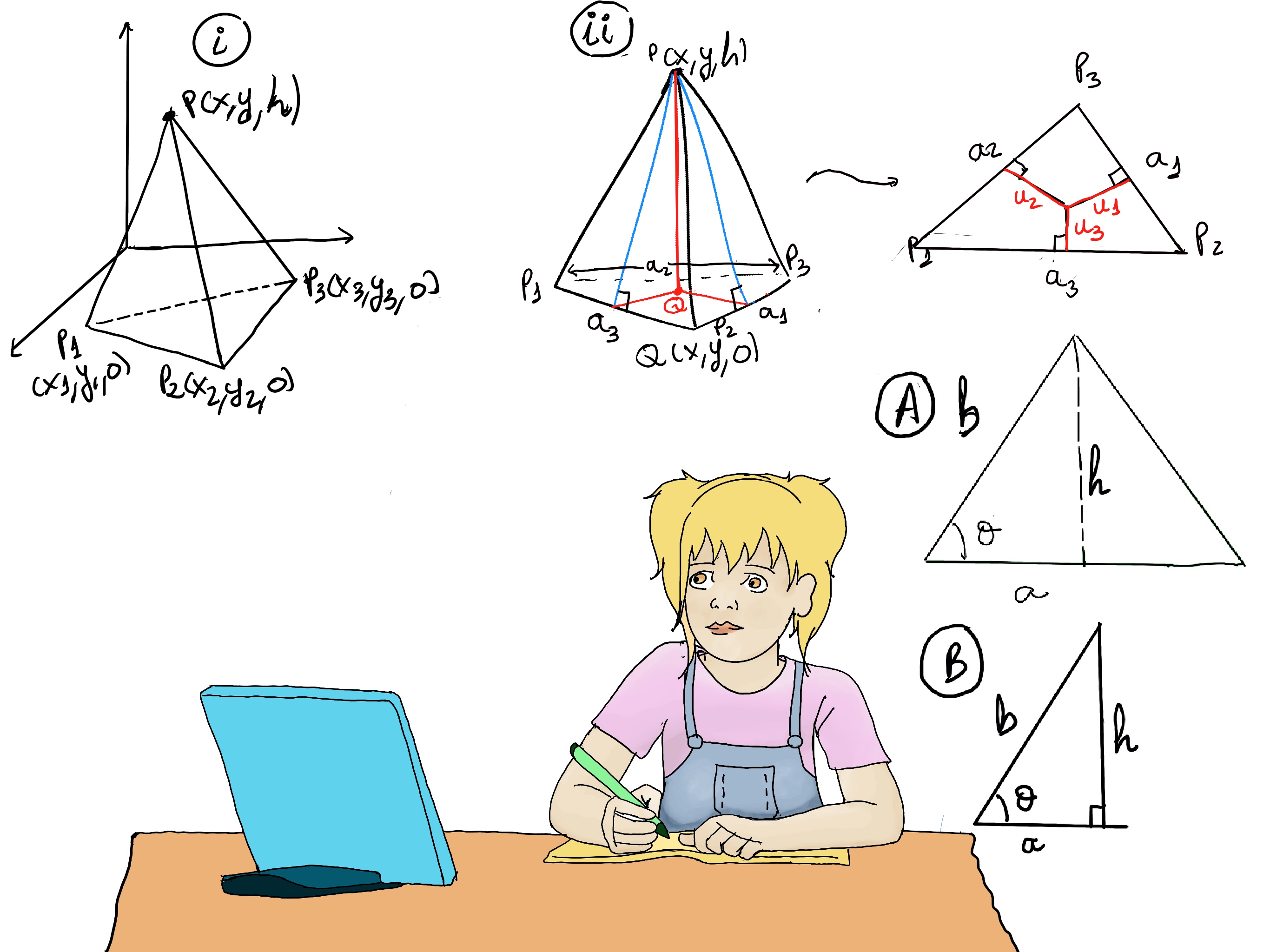
Of course, the volume equals ¹⁄₃Area(base)·height, and so we are told the volume and the area are fixed, hence the height h is fixed.

Let u₁, u₂, and u₃ be the distances from Q to sides where Q(x, y, 0) and the peak P(x, y, h).

Minimize the total surface area is the same problem ↭ minimize the area of the three triangles (the area of the base is fixed) with heights $\sqrt{u_1^2+h^2}, \sqrt{u_2^2+h^2}, \sqrt{u_3^2+h^2} ⇒ SideArea = f(u_1, u_2, u_3) = \frac{1}{2}a_1\sqrt{u_1^2+h^2}+\frac{1}{2}a_2\sqrt{u_2^2+h^2}+\frac{1}{2}a_3\sqrt{u_3^2+h^2}$ and the constraint is Area(base) = g(u_1, u_2, u_3) = constant. Each of these sides have base $\frac{1}{2}a_1u_1, \frac{1}{2}a_2u_2,~ and~ \frac{1}{2}a_3u_3$ respectively, so the total Area(base) = $\frac{1}{2}a_1u_1 + \frac{1}{2}a_2u_2 + \frac{1}{2}a_3u_3$

∇f = λ ∇fg: $\frac{∂f}{u_1} = \frac{1}{2}a_1\frac{u_1}{\sqrt{u_1^2+h^2}}, \frac{∂f}{u_2} = \frac{1}{2}a_2\frac{u_2}{\sqrt{u_2^2+h^2}}, \frac{∂f}{u_3} = \frac{1}{2}a_3\frac{u_3}{\sqrt{u_3^2+h^2}}, \frac{∂g}{u_1} = \frac{1}{2}a_1, \frac{∂g}{u_2} = \frac{1}{2}a_2, \frac{∂g}{u_3} = \frac{1}{2}a_3$ ⇒[∇f = λ ∇fg] $ \frac{∂f}{u_1} = \frac{1}{2}a_1\frac{u_1}{\sqrt{u_1^2+h^2}} = λ\frac{1}{2}a_1 ↭ \frac{u_1}{\sqrt{u_1^2+h^2}} = λ,$ and similarly, $\frac{u_2}{\sqrt{u_2^2+h^2}} = λ, \frac{u_3}{\sqrt{u_3^2+h^2}} = λ ⇒ \frac{∂f}{u_1} = \frac{1}{2}a_1\frac{u_1}{\sqrt{u_1^2+h^2}} = λ, \frac{∂f}{u_2} = λ, \frac{∂f}{u_3} = λ$

The solution to the system $\frac{∂f}{u_1} = \frac{∂f}{u_2} = \frac{∂f}{u_3} = λ$ is u₁ = u₂ = u₃ ⇒ Q is the incenter.

Recall that the incenter is the point where the three interior angle bisectors of a triangle meet. The incenter is equidistant from the sides of the triangle.

Non-independent variables

In multivariable calculus, when dealing with functions of multiple variables, there are often situations where some variables are not independent of each other. Instead, they may be related by equations or constraints, e.g., let f(x, y, z) be a multivariable function where g(x, y, z) = c where c is a constant, we can often solve for one of the variables in term of the others and, of course, we want to understand how these variables are related to each other.

Consider the function f(x, y, z) = x² + y² + z² and the constraint g(x, y, z) = x + y + z = 1, we can solve the constraint equation for one variable, z = z(x, y) = 1 -x -y, so we can compute $\frac{∂f}{∂y}, \frac{∂f}{∂y}$.

Example. x² + yz + z³ = 8 at (2, 3, 1).

Recall that the total differential df of a multivariable function f(x, y, z) is given by df = $\frac{∂f}{∂y}dx + \frac{∂f}{∂y}dy + \frac{∂f}{∂z}dz$ where $\frac{∂f}{∂x} = 2x, \frac{∂f}{∂y} = z, \frac{∂f}{∂z} = y + 3z^2 ⇒df = 2xdx + zdy + (y+3z^2)dz = 8$ because 8 is a constant (g(x, y, z) = constant, df is obviously zero).

When differentiating with respect to a particular variable, we treat all other variables as constants.

$df = 2xdx + zdy + (y+3z^2)dz = 8$ at (2, 3, 1) results in 4dx + dy + 6dz = 0⇒$dz = \frac{-1}{6}(4dx +dy)$ ⇒[z = z(x, y), dz = $\frac{∂z}{∂z}dx + \frac{∂z}{∂y}dz$] $\frac{∂z}{∂z} = \frac{-4}{6} = \frac{-2}{3}, \frac{∂z}{∂y} = \frac{-1}{6}$

As we previously stated, when differentiating with respect to a particular variable, we treat all other variables as constants, $\frac{∂z}{∂z} =$[y is constant, hence dy = 0, $dz = \frac{-1}{6}(4dx +dy)$] $\frac{-4}{6} = \frac{-2}{3}$.

In the general case, g(x, y, z) = c, then $dg = \frac{∂g}{∂x}dx + \frac{∂g}{∂y}dy + \frac{∂g}{∂z}dz =[\text{In a different notation}] g_xdx + g_ydy + g_zdz = 0$ ⇒[Solve for dz] $dz = -\frac{g_x}{g_z}dx -\frac{g_y}{g_z}dy$. In a similar fashion, $\frac{∂z}{∂x}$ = [Set y = constant which implies dy = 0, and substituting gy = 0 ⇒dz = $-\frac{g_x}{g_z}dx$] $-\frac{g_x}{g_z}, \frac{∂z}{∂x} = -\frac{g_x}{g_y}$.

This could become a little confusing, e.g., f(x, y) = x + y, $\frac{∂f}{∂x} =1$, and let’s consider a change of variables x = u, y = u + v, then f(x, y) = x + y = 2u +v, so $\frac{∂f}{∂x} =1, \frac{∂f}{∂u} = 2$ but x = u!!! This is not a contradiction, because when we take the partial derivate of a function f(x, y) with respect to x, $\frac{∂f}{∂x}$, we are asking how f changes as we vary x while holding y constant. Similarly, when we take the partial derivate of a function f(u, v) with respect to u, $\frac{∂f}{∂u} = 1$ we are asking how f changes as we vary u while holding v constant.

Therefore, these notation can become confusing because they don’t make explicit what variable are being hold constant, we could clarify our previous notation, $(\frac{∂f}{∂x})_y$ that explicitly states that the partial derivative is taken with respect to x while holding y constant⇒ Assume f = f(x, y, z) where g(x, y, z) = c, $(\frac{∂f}{∂x})_y$ is the rate of change of f with respect to x, y = constant, x varies, and z =z(x, y). It provides clarity and eliminates ambiguity, but it is not especially pleasing to the eye 😄; and $(\frac{∂f}{∂u})_v$ states that the partial derivative is taken with respect to u while holding v constant.

Using this notation, it is clearly obvious that $(\frac{∂f}{∂x})_y = 1 ≠ (\frac{∂f}{∂x})_v = (\frac{∂f}{∂u})_v = 2$

Exercise

• Calculate the area of a triangle (Figure A).

Area = $\frac{1}{2}a·h = \frac{1}{2}a·b·sin(θ)$, so A = A(a, b, θ).

Let’s add a constrain and suppose that is a right triangle (Figure B) ⇒ a = b·cos(θ).

What is the rate of change of A with respect to θ?

• We can consider a, b, θ as independent variables: $\frac{∂A}{∂θ} = (\frac{∂A}{∂θ})_{a b}$.

$\text{However, this is not possible because then the triangle would not be a right triangle}, \frac{∂A}{∂θ} = (\frac{∂A}{∂θ})_{a, b} = \frac{1}{2}a·b·cos(θ).$

• We can keep a constant, so b will change b (θ also changes) = b(a, θ) = $\frac{a}{cos(θ)}$ and we keep the right triangle constrain, $(\frac{∂A}{∂θ})_a$

• We can keep b constant, so a will change a = a(b, θ) = $\frac{b}{sin(θ)}$ and we keep the right triangle constrain, $(\frac{∂A}{∂θ})_b$

Let’s calculate $(\frac{∂A}{∂θ})_a$ where A = $\frac{1}{2}a·b·sin(θ)$ and a = b·cos(θ).

In this particular case (it is not a general method by any means), we can solve for b, that is, a = b·cos(θ) ⇒b = $\frac{a}{cos(θ)} = a·sec(θ)$ and substitute, so A = $\frac{1}{2}a·b·sin(θ) = \frac{1}{2}a^2·sin(θ)·sec(θ) = \frac{1}{2}a^2·\frac{sin(θ)}{cos(θ)} =\frac{1}{2}a^2·tan(θ) ⇒ (\frac{∂A}{∂θ})_a = \frac{1}{2}a^2·sec^2(θ)$.

The general method is to take differentials considering that a is fixed (da = 0). Our constrain is a = b·cos(θ) ⇒[Product rule] da = cos(θ)db -bsin(θ)dθ ⇒ 0 = cos(θ)db -bsin(θ)dθ ⇒ cos(θ)db =bsin(θ)dθ ⇒ db = btan(θ)dθ

A = $\frac{1}{2}a·b·sin(θ)⇒$[Recall that the total differential df of a multivariable function A(a, b, θ) is given by dA = $\frac{∂A}{∂a}da + \frac{∂A}{∂b}db + \frac{∂A}{∂θ}dθ$] = $\frac{1}{2}·b·sin(θ)·da+\frac{1}{2}·a·sin(θ)·db+\frac{1}{2}abcos(θ)dθ$ =[da = 0, db = btan(θ)dθ] $da = \frac{1}{2}·a·sin(θ)·btan(θ)dθ+\frac{1}{2}abcos(θ)dθ = \frac{1}{2}ab(sin(θ)tan(θ)+cos(θ))dθ = \frac{1}{2}ab(\frac{sin^2(θ)}{cos(θ)}+cos(θ))dθ = \frac{1}{2}ab(\frac{sin^2(θ)+cos^2(θ)}{cos(θ)})dθ = \frac{1}{2}ab(\frac{1}{cos(θ)})dθ = \frac{1}{2}absec(θ)dθ$

$ dA = \frac{1}{2}absec(θ)dθ ⇒ (\frac{∂A}{∂θ})_a$ =[dA = $\frac{∂A}{∂a}da + \frac{∂A}{∂b}db + \frac{∂A}{∂θ}dθ$] $\frac{1}{2}absec(θ)$

The idea is to write dA in terms of da, db, and dθ, set da = 0 (a = constant), and differentiate the constraint, so we can solve for db in terms of dθ and plug it into dA so we can get the answer.

Another method is to apply the chain rule, $(\frac{∂A}{∂θ})_a = \frac{∂A}{∂θ}(\frac{∂θ}{∂θ})_a + \frac{∂A}{∂a}(\frac{∂a}{∂θ})_a + \frac{∂A}{∂b}(\frac{∂b}{∂θ})_a = A_θ(\frac{∂θ}{∂θ})_a + A_a(\frac{∂a}{∂θ})_a + A_b(\frac{∂b}{∂θ})_a =$[where A = A(a, b, θ), $A_θ = \frac{∂A}{∂θ}$, the rate of change of A with respect to θ when we hold all other variables constant. It seems complicated, but $(\frac{∂θ}{∂θ})_a=1, (\frac{∂θ}{∂θ})_a = 0$ since a is constant] = $A_b(\frac{∂b}{∂θ})_a$ and we need to use the constrain to calculate this term.

Calculate $(\frac{∂f}{∂z})_y$

f = f(x, y, z), constrain g(x, y, z) = 0, y constant, x varies, x = x(y, z)

1st method. To calculate $(\frac{∂f}{∂z})_y$ where y = constant, x varies, x = x(y, z) using differentials, df = $\frac{∂f}{∂x}dx + \frac{∂f}{∂y}dy + \frac{∂f}{∂z}dz = f_xdx + f_ydy + f_zdz = f_xdx + f_zdz$. Futhermore, g(x, y, z) = 0⇒ dg = $g_xdx + g_ydy + g_zdz = 0 ⇒$[y = constant ⇒ g_y = 0] $dx = \frac{-g_z}{g_x}dz$ and this is the rate of change of x with respect to z when we keep y constant, i.e., $(\frac{∂x}{∂z})_y = \frac{-g_z}{g_x}dz$.

Next, we plug this one in the previous equation, df = $f_xdx + f_zdz = f_x\frac{-g_z}{g_x}dz + f_zdz = (f_x\frac{-g_z}{g_x} + f_z)dz$, hence $(\frac{fx}{∂z})_y = f_x\frac{-g_z}{g_x} + f_z$.

2nd method.

$(\frac{∂f}{∂z})_y =$[Chain Rule] $\frac{∂f}{∂x}(\frac{∂x}{∂z})_y+\frac{∂f}{∂y}(\frac{∂y}{∂z})_y+\frac{∂f}{∂z}(\frac{∂z}{∂z})_y$ =[$(\frac{∂y}{∂z})_y = 0, (\frac{∂z}{∂z})_y=1$] $\frac{∂f}{∂x}(\frac{∂x}{∂z})_y+\frac{∂f}{∂z}$

g(x, y, z) = 0⇒ $0 = (\frac{∂g}{∂z})_y = \frac{∂g}{∂x}(\frac{∂x}{∂z})_y+\frac{∂g}{∂y}(\frac{∂y}{∂z})_y+\frac{∂g}{∂z}(\frac{∂z}{∂z})_y = \frac{∂g}{∂x}(\frac{∂x}{∂z})_y+\frac{∂g}{∂z} ⇒0 = \frac{∂g}{∂x}(\frac{∂x}{∂z})_y+\frac{∂g}{∂z} = g_x(\frac{∂x}{∂z})_y+g_z ⇒ (\frac{∂x}{∂z})_y = \frac{-g_z}{g_x}$, and yet again we plug this in the previous equation, $(\frac{∂f}{∂z})_y = \frac{∂f}{∂x}(\frac{∂x}{∂z})_y+\frac{∂f}{∂z} = \frac{∂f}{∂x}\frac{-g_z}{g_x}+\frac{∂f}{∂z} = f_x\frac{-g_z}{g_x} + f_z$, so both method are essentially the same.

Partial differential equation

A partial differential equation is an equation involving an unknown function of several variables and its partial derivatives with respect to those variables.

The heat equation describes how heat diffuses through a medium over time. It is a classic example of a partial differential equation, $\frac{∂f}{∂t} = k(\frac{∂^2f}{∂x^2}+\frac{∂^2f}{∂y^2}+\frac{∂^2f}{∂z^2})\text{where}\frac{∂f}{∂t}$ represents the rate of change of temperature with respect to time and f = f(x, y, z, t); k is the thermal diffusivity, a constant that characterizes how quickly heat spreads through the material, and $\frac{∂^2f}{∂x^2}$ is the spatial variation of temperature (second derivative with respect to position), i.e., the rate of change of temperature at any point is proportional to the second derivative of temperature with respect to space.

Double integrals

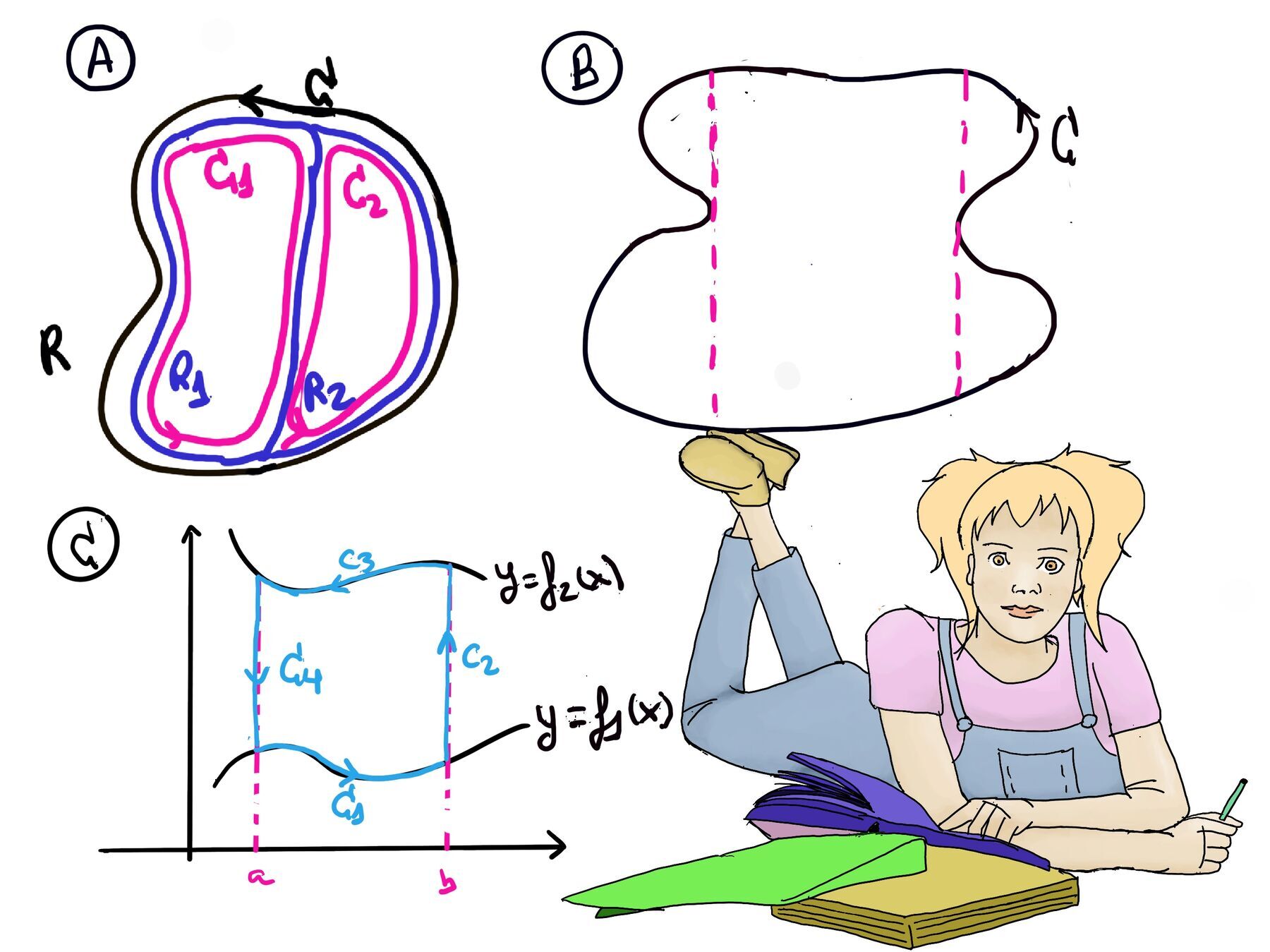
The definite integral of a function f(x), denoted as $\int_{a}^{b} f(x)dx$, will give you the signed area between the graph of the function and the x-axis over [a, b], that is, we subtract area below the x-axis from the area above the x-axis.

A double integral is an integral that integrates a function of two variables over a region R in a two-dimensional space. It represents the volume under a surface, that is, the volume below the graph z = f(x, y).

It is denoted as $\iint_R f(x, y) dA$ Where R is the region over which the integration is performed; f(x,y) is the integrand, representing the function being integrated; and dA represents an infinitesimal area element in the region R.

Obviously, the formal definition will be reduced R into small pieces ΔA_i and we will consider the sum $\sum_{i} f(x_i, y_i)ΔA_i$ and take the limits as ΔA_i→ 0.

Loosely speaking, to compute this integral, you would typically set up the limits of integration, perform the integration with respect to x, take slices (S(x) is the area of slice by yz-planes), so the volume would be $\int_{x_{min}}^{x_{max}} S(x)dx$. Then, S(x) = $\int_{y_{min(x)}}^{y_{max(x)}} f(x, y)dy$, hence $\iint_R f(x, y) dA\ = \int_{x_{min}}^{x_{max}} [\int_{y_{min(x)}}^{y_{max(x)}} f(x, y)dy]dx$

Bibliography

1. NPTEL-NOC IITM, Introduction to Galois Theory.
2. Algebra, Second Edition, by Michael Artin.
3. LibreTexts, Calculus and Calculus 3e (Apex). Abstract and Geometric Algebra, Abstract Algebra: Theory and Applications (Judson).
4. Field and Galois Theory, by Patrick Morandi. Springer.
5. Michael Penn, and MathMajor.
6. Contemporary Abstract Algebra, Joseph, A. Gallian.
7. YouTube’s Andrew Misseldine: Calculus. College Algebra and Abstract Algebra.
8. MIT OpenCourseWare 18.01 Single Variable Calculus, Fall 2007 and 18.02 Multivariable Calculus, Fall 2007.
9. Calculus Early Transcendentals: Differential & Multi-Variable Calculus for Social Sciences.