Gradient vector

And there are never really endings, happy or otherwise. Things keep going on, they overlap and blur, your story is part of your sister’s story is part of many other stories, and there is no telling where any of them may lead. Everything turns in circles and spirals with the cosmic heart until infinity.

Gradient vector

The Chain Rule w = f(x, y, z) where x = x(t), y = y(t), and z = z(t) are functions of another variable t, then the derivate of f with respect to t is given by $\frac{dw}{dt} = f_x\frac{dx}{dt} +f_y\frac{dy}{dt}+f_z\frac{dz}{dt}, \frac{dw}{dt} = w_x\frac{dx}{dt} +w_y\frac{dy}{dt}+w_z\frac{dz}{dt} = ∇w·\frac{d\vec{r}}{dt}~$ where ∇w = ⟨w_x, w_y, w_z⟩ and $\frac{d\vec{r}}{dt}=⟨\frac{d\vec{x}}{dt}, \frac{d\vec{y}}{dt}, \frac{d\vec{z}}{dt}⟩$

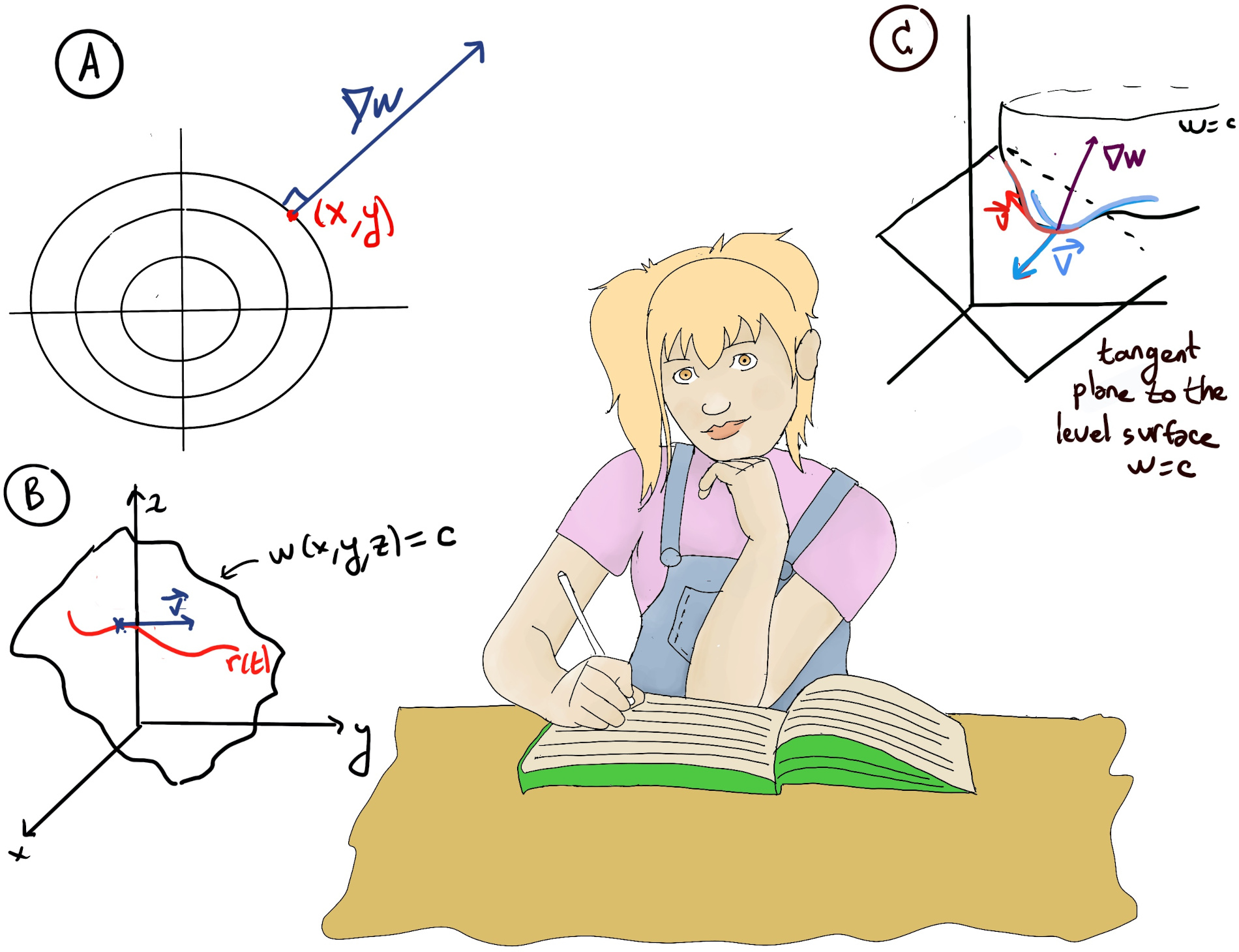
The gradient vector is defined as follows: ∇w = ⟨w_x, w_y, w_z⟩ = $⟨\frac{\partial w}{\partial x}, \frac{\partial w}{\partial y}, \frac{\partial w}{\partial z}⟩$. It is a vector that points in the direction of the steepest increase of a function at a given point, e.g., w = a₁x + a₂y + a₃z, ∇w = ⟨a₁, a₂, a₃⟩.

Theorem. The gradient vector is perpendicular to the level surfaces of the function. Since the gradient points in the direction of maximum increase, it must be perpendicular to the level surface, as there is no change in the function’s value in that direction.

Recall that for a given constant c, the level surface of f is the set of points (x, y, z) such that f(x,y,z) = c. In our particular case, w = a₁x + a₂y + a₃z = c. Futhermore, we already know that a₁x + a₂y + a₃z is a plane with normal vector ⟨a₁, a₂, a₃⟩, that is, the gradient vector.

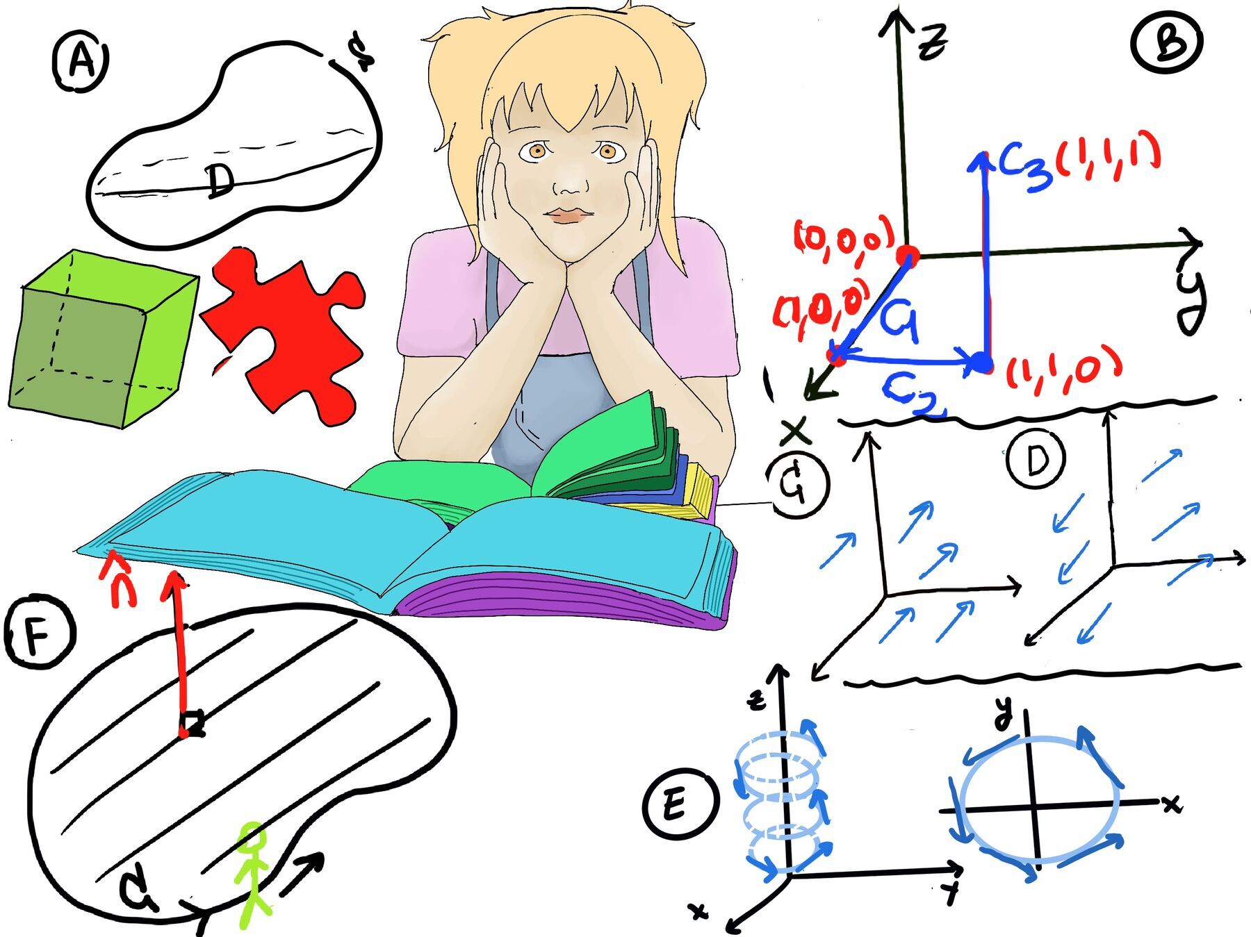
Let’s see this theorem in another example. w = x² + y², the level surfaces, w = c = x² + y² are circles, ∇w = ⟨2x, 2y⟩ is perpendicular to the level surface (Figure A).

Proof.

Let’s take a curve $\vec{r} = \vec{r}(t)$ that stays on the level surface, w(x, y, z) = c (Figure B). The velocity vector of this motion ($\vec{r}$) is tangent to the level surface, and therefore, is tangent to the surface w = x (it is obvious because the curve lives on the surface), $\vec{v} = \frac{d\vec{r}}{dt}$.

By the chain rule, $\frac{dw}{dt} = ∇w·\frac{d\vec{r}}{dt} = ∇w·\vec{v}$ =[The curve $\vec{r}$ stays on the level surface w = c, $\frac{d\vec{r}}{dt}=⟨\frac{d\vec{x}}{dt}, \frac{d\vec{y}}{dt}, \frac{d\vec{z}}{dt}⟩ = 0$ since w(t) = c] 0 ⇒[if the dot product of two vectors is zero, then the two vectors are perpendicular, or orthogonal, to each other] ∇w ⊥ $\vec{v}$, and this is true for any motion on w = c, that is, $\vec{v}$ can be any vector tangent to w = c (Figure C), hence the gradient vector is perpendicular to the level surface ∎

Exercise: Find the tangent plane to the surface x² + y² -z² = 4 at (2, 1, 1).

The level set is w = 4 where w = x² + y² -z², ∇w = $⟨2x, 2y, -2z⟩\bigg|_{(2, 1, 1)}$ =⟨4, 2, -2⟩ is normal to the surface, so the equation’s surface is 4x +2y -2z =[4·2+2·1+-2·1] 8

Another way of solving this exercise is as follows, dw = 2xdx + 2ydy -2zdz =[(2, 1, 1)] 4dx + 2dy -2dz ⇒Δw ≈ 4Δx + 2Δy -2Δz

The tension plane is 4(x-2) +2(y-1) -2(z-1) = 0.

The gradient vector is perpendicular to the level surfaces of the function where the function has a constant value (w = f(x, y, z) = c). The tension plane is the plane perpendicular to the gradient vector at a specific point on the surface. The gradient vector ∇f(x₀, y₀, z₀) gives the direction of the tension plane, and the equation of the tension plane passing through x₀, y₀, z₀ is the dot product (indicating orthogonality) ∇f(x₀, y₀, z₀)(x -x₀, y -y₀, z -z₀)=0

Directional derivatives

Directional derivatives represents how a function w = w(x, y) changes as you move in a specific direction from a point in its domain.

$\frac{\partial w}{\partial x}, \frac{\partial w}{\partial y}$ generalize the notion of a derivative, which in single-variable calculus represents the rate of change of the function with respect to one variable. Thus, in the context of function of two or more variables, $\frac{\partial w}{\partial x}, \frac{\partial w}{\partial y}$ represent the derivate of f in the direction of $\vec{i}, \vec{j}$ respectively.

More generally, we might be interested in knowing how the function changes not just along the traditional coordinate axes but in any arbitrary direction, so given a function f: ℝⁿ → ℝ and a point “a” in its domain, the directional derivate of f at “a” in the direction of a unit vector $\vec{u}$ = ⟨a, b⟩ (a vector in ℝⁿ that has a length of 1). In other words, we are asking what is going on if we move linearly in the direction of $\vec{u}$ (Figures A and B), say a position vector $\vec{r(s)}$ where $\frac{d\vec{r}}{ds}=\vec{u}$, that is, $\frac{dw}{ds}\bigg|_{\vec{u}}$. This is the slope of a slice (blue) of the graph by a vertical plane parallel to ${\vec{u}}$

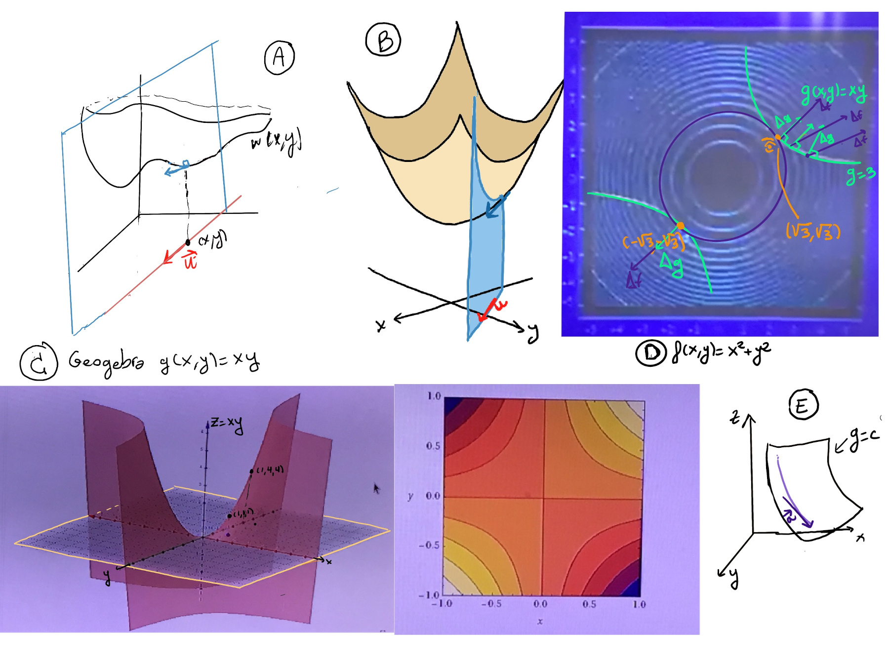
$\vec{u}$ = ⟨a, b⟩, then x(x) = x₀ + as, y(s) = y₀ + bs.

We know $\frac{dw}{ds}\bigg|_{\vec{u}} = ∇w·\frac{d\vec{r}}{ds}$ =[We are moving a unit speed in the direction of $\vec{u}$] ∇w·$\vec{u}$

Example: $\frac{dw}{ds}\bigg|_{\vec{i}} = ∇w·\vec{i} = ⟨\frac{\partial w}{\partial x}, \frac{\partial w}{\partial y}, \frac{\partial w}{\partial z}⟩·\vec{i} = \frac{\partial w}{\partial x}$.

Geometrically, $\frac{dw}{ds}\bigg|_{\vec{u}} = ∇w·\vec{u} = |∇w|·|\vec{u}|cos(θ) = |∇w|·cos(θ)$, and this value is largest when cos(θ) = 1 ↭ θ = 0, that means, $\vec{u}$ is in the direction of the gradient ∇w.

The gradient points in the direction of the greatest or fastest increase of f (or w, or whatever 😄), that is, the direction of the steepest ascent at a given point, and |∇w| = $\frac{dw}{ds}\bigg|_{\vec{u}=dir(∇w)}$.

Conversely, $\frac{dw}{ds}\bigg|_{\vec{u}}$ is minimal when cos(θ) = -1 ↭ θ = 180, that is, $\vec{u}$ is in the opposite direction of the gradient ∇w.

Futhermore, $\frac{dw}{ds}\bigg|_{\vec{u}} = 0$,the function w does not change. In other words, we are moving along a surface level or contour line of w ↭ cos(θ) = 0 ↭ θ = 90° ↭ $\vec{u}$ ⊥ ∇w, that is, the direction of movement ($\vec{u}$) is perpendicular to the direction of maximum change (∇w).

Bibliography

1. NPTEL-NOC IITM, Introduction to Galois Theory.
2. Algebra, Second Edition, by Michael Artin.
3. LibreTexts, Calculus and Calculus 3e (Apex). Abstract and Geometric Algebra, Abstract Algebra: Theory and Applications (Judson).
4. Field and Galois Theory, by Patrick Morandi. Springer.
5. Michael Penn, and MathMajor.
6. Contemporary Abstract Algebra, Joseph, A. Gallian.
7. YouTube’s Andrew Misseldine: Calculus. College Algebra and Abstract Algebra.
8. MIT OpenCourseWare 18.01 Single Variable Calculus, Fall 2007 and 18.02 Multivariable Calculus, Fall 2007.
9. Calculus Early Transcendentals: Differential & Multi-Variable Calculus for Social Sciences.