Functions of two variables.

Functions of two variables

Functions of two variables are natural generalizations of functions of one variable. They are mathematical functions f: ℝ x ℝ → R associating to each pair of real numbers (x, y) a third real number f(x, y), i.e., they take two inputs and produce one output. Such a function assigns to each ordered pair of its domain, a unique real number.

They are typically denoted by f(x,y), where x and y are the two variables, e.g., f(x, y) = 2x + 3y, f(x, y) = x² + y², e^x+y, etc.

Their domain is the set of all possible input values for both variables x and y, e.g., f(x, y) = $\sqrt{x+y}$, Domain(f) = {x, y ∈ ℝ x ℝ : x + y ≥ 0}, f(x, y) = $\frac{1}{x+y}$, Domain(f) = {x, y ∈ ℝ x ℝ : x + y ≠ 0}

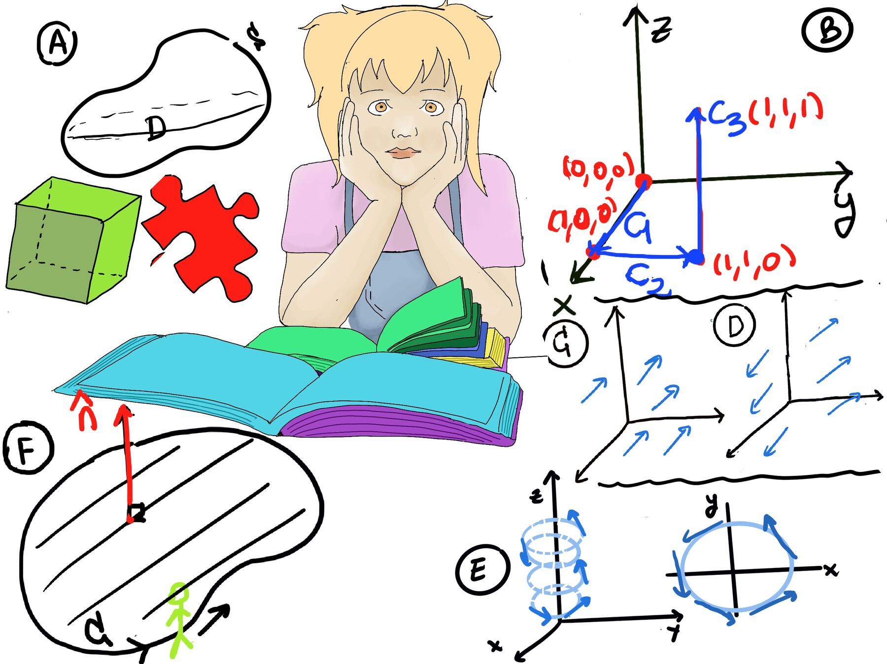
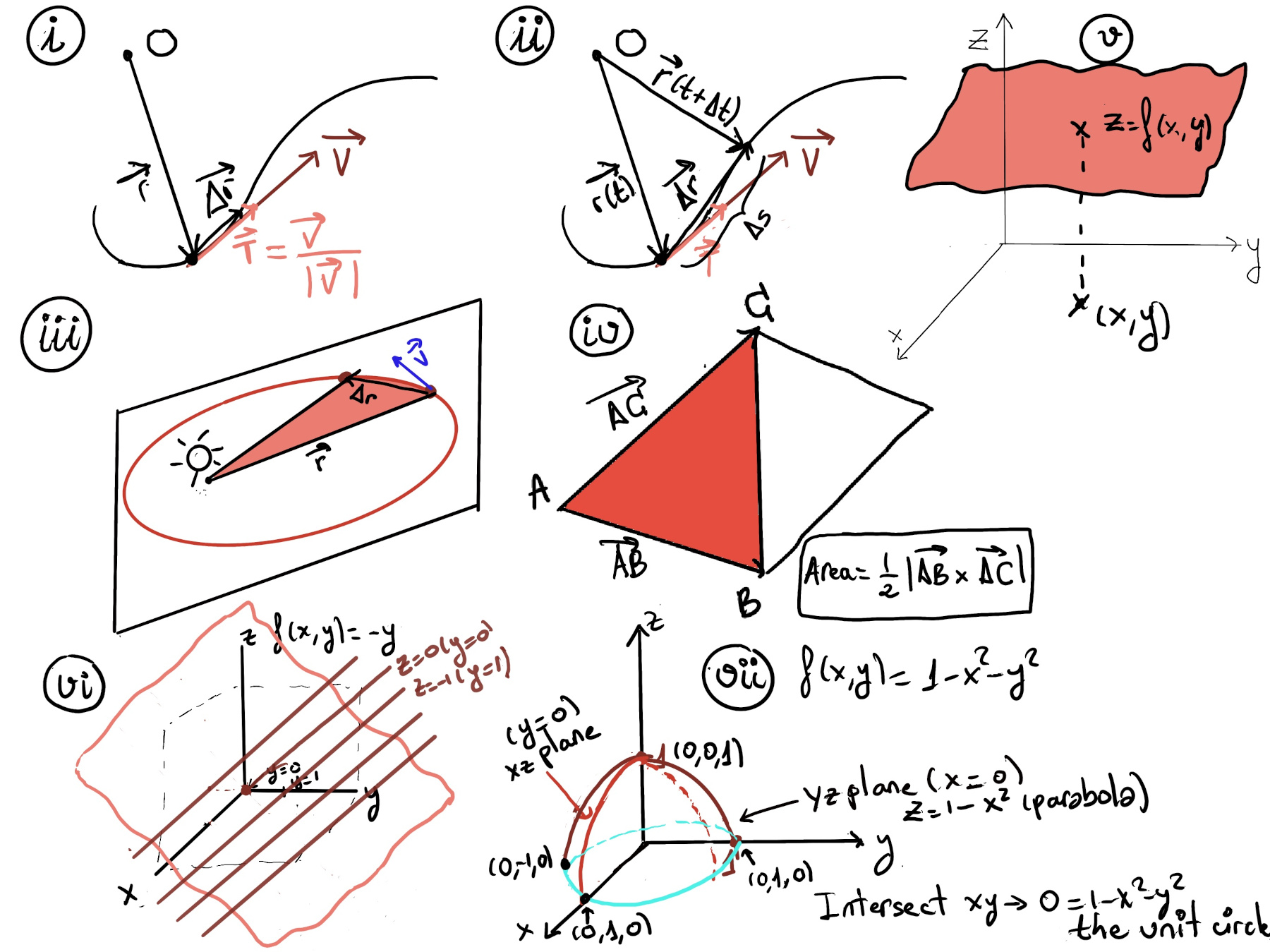
The graph of a two-variable function is usually a surface in a Cartesian space (Figure v), e.g. f(x, y) = -y (Figure vi), f(x, y) = 1 -x² -y² (Figure vii. Notice that in the yz plane, x = 0, z = 1 -y², that is, a parabola), and z = y² -x² (Figure i).

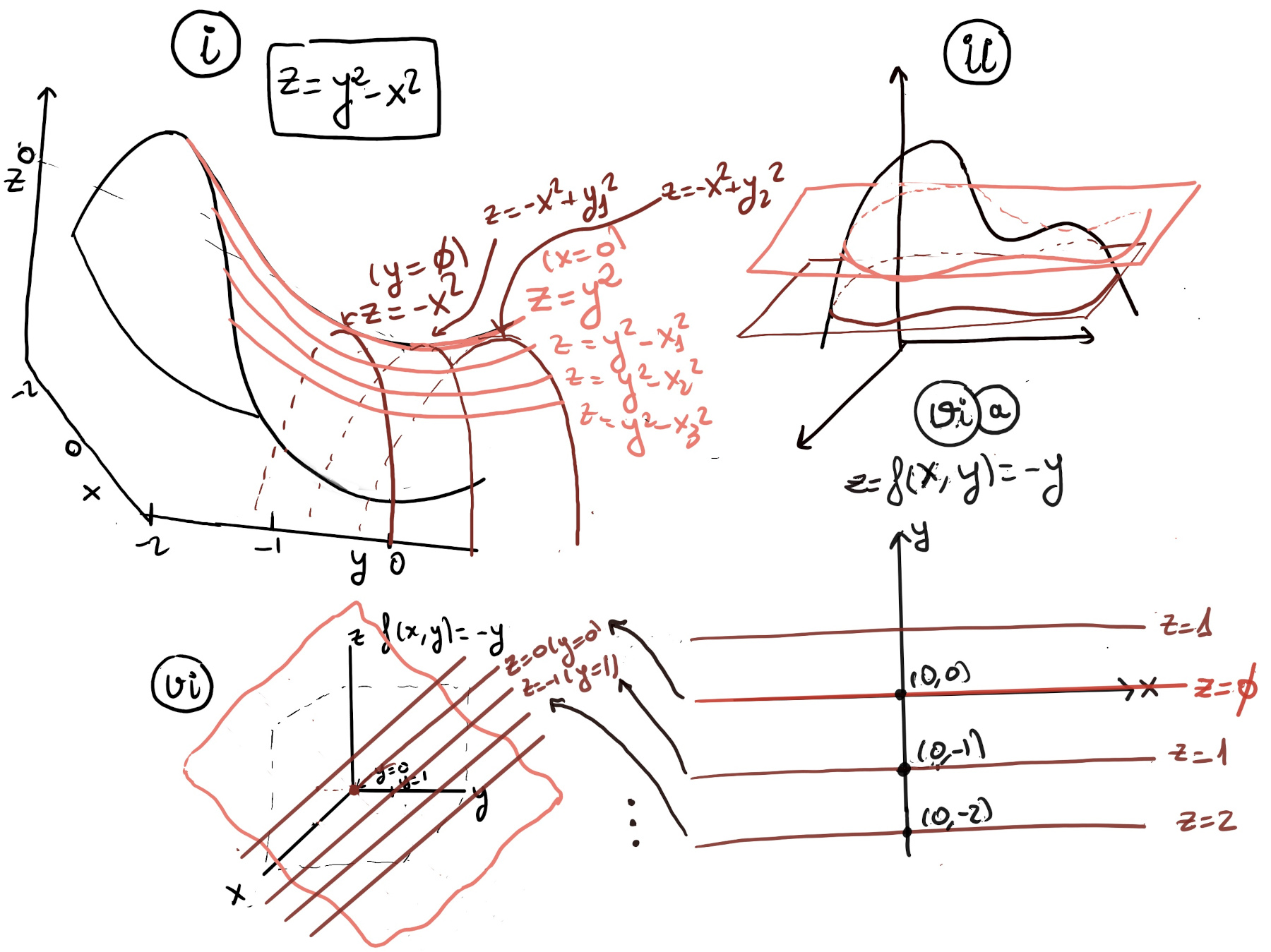
Contour plots are used to show 3-dimensional data on a 2-dimensional surface. It is like a topographical map in which x-, y-, and z-values are plotted instead of longitude, latitude, and elevation. A synoptic chart is the scientific term for a weather map. Contour lines on topographic maps connect points of equal altitude, while isobars connect points which share the same atmospheric (air) pressure.

A contour plot shows all the points where z = f(x, y) equals some fixed constant, chosen at regular intervals (Figure ii), e.g., Figure via, Figure ia, Figure viia. Please observe that in the last contour plots the level curves are getting closer and closer, so the function is getting steeper and steeper (thinking about it or picture it like a mountain)

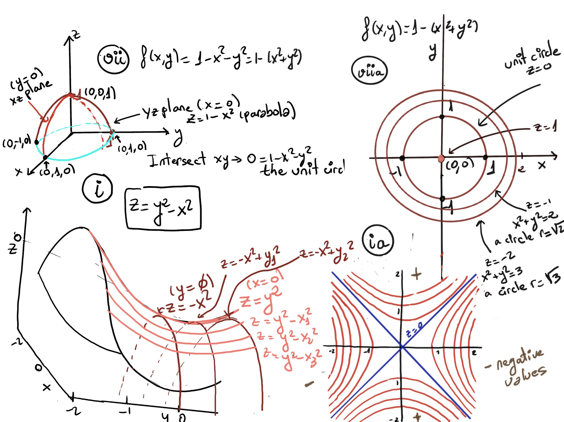
A level curve is simply a cross section of the graph of z=f(x,y) taken at a constant value, say z=c. A level curve can be interpreted as a contour line on a map, where each line represents points with the same elevation.

Bibliography

1. NPTEL-NOC IITM, Introduction to Galois Theory.
2. Algebra, Second Edition, by Michael Artin.
3. LibreTexts, Calculus and Calculus 3e (Apex). Abstract and Geometric Algebra, Abstract Algebra: Theory and Applications (Judson).
4. Field and Galois Theory, by Patrick Morandi. Springer.
5. Michael Penn, and MathMajor.
6. Contemporary Abstract Algebra, Joseph, A. Gallian.
7. YouTube’s Andrew Misseldine: Calculus. College Algebra and Abstract Algebra.
8. MIT OpenCourseWare 18.01 Single Variable Calculus, Fall 2007 and 18.02 Multivariable Calculus, Fall 2007.
9. Calculus Early Transcendentals: Differential & Multi-Variable Calculus for Social Sciences.