Double integrals

Give me six hours to chop down a tree and I will spend the first four sharpening the axe, Abraham Lincoln.

Double integrals

The definite integral of a function f(x), denoted as $\int_{a}^{b} f(x)dx$, will give you the signed area between the graph of the function and the x-axis over [a, b], that is, we subtract area below the x-axis from the area above the x-axis.

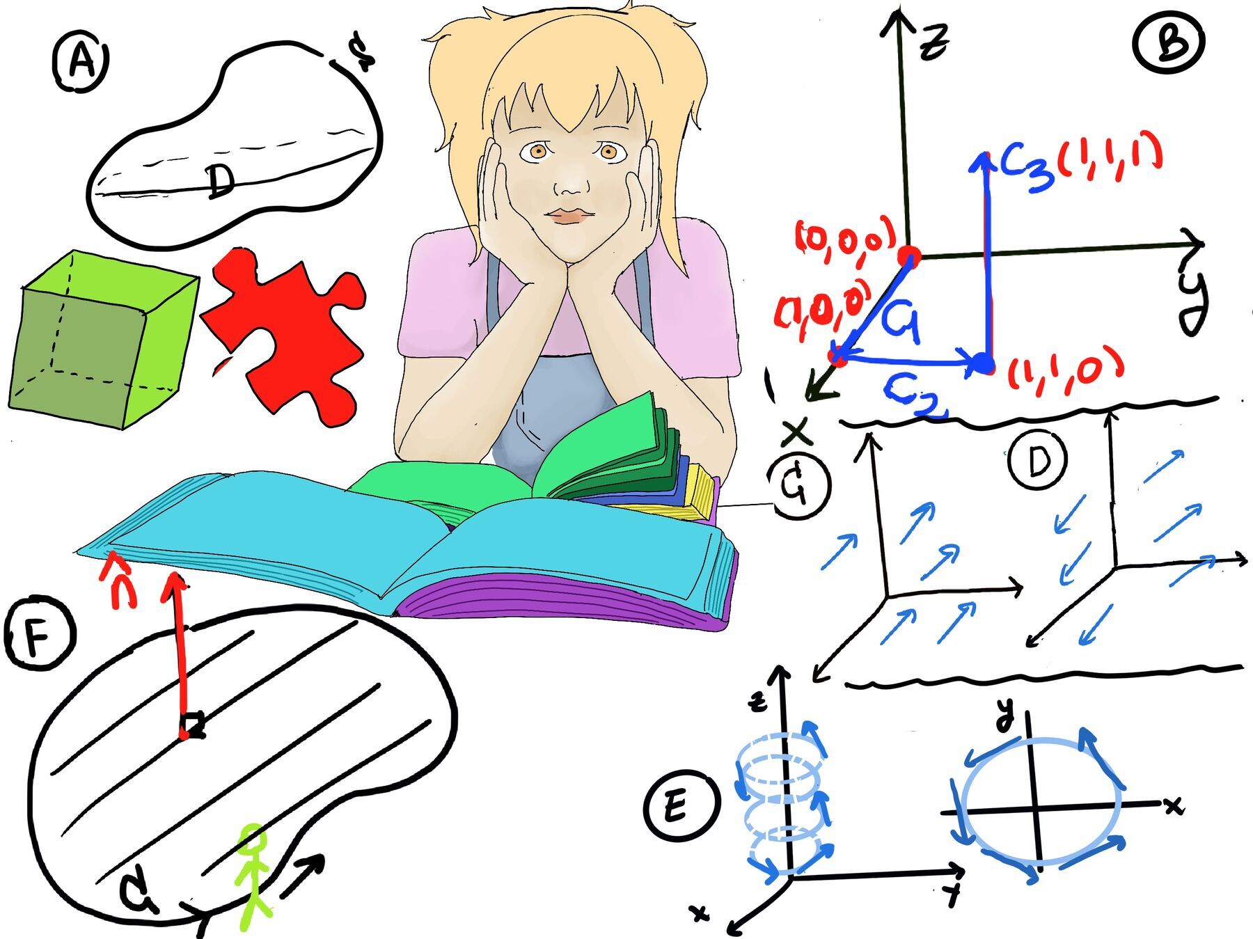
A double integral is an integral that integrates a function of two variables over a region R in a two-dimensional space. It represents the volume under a surface, that is, the volume below the graph z = f(x, y) (Figure 1).

It is denoted as $\iint_R f(x, y) dA$ Where R is the region over which the integration is performed; f(x,y) is the integrand, representing the function being integrated; and dA represents an infinitesimal area element in the region R (Figure 2).

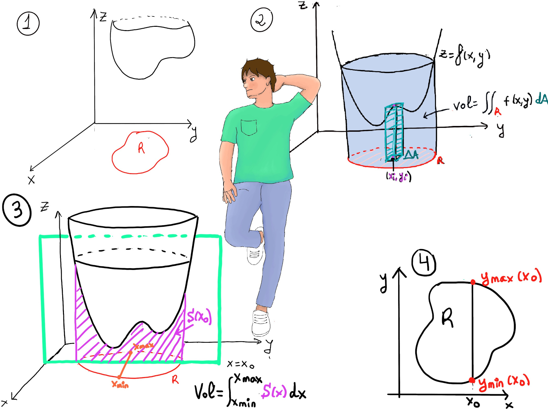
Obviously, the formal definition will be reduced R into small pieces ΔA_i and we will consider the sum $\sum_{i} f(x_i, y_i)ΔA_i$ and take the limits as ΔA_i→ 0 (Figure 3).

Loosely speaking, to compute this integral, you would typically set up the limits of integration, perform the integration with respect to x, take slices (S(x) is the area of slice by yz-planes), so the volume would be $\int_{x_{min}}^{x_{max}} S(x)dx$. Then, S(x) = $\int_{y_{min(x)}}^{y_{max(x)}} f(x, y)dy$, hence $\iint_R f(x, y) dA\ = \int_{x_{min}}^{x_{max}} [\int_{y_{min(x)}}^{y_{max(x)}} f(x, y)dy]dx$ (Figure 4).

Solved examples

• Let z = f(x, y) = 1 -x² -y² and the region is determined by 0 ≤ x ≤ 1, 0 ≤ y ≤ 1 (Figure A, B, and C), please notice that f(0.9, 0.9) = -0.62.

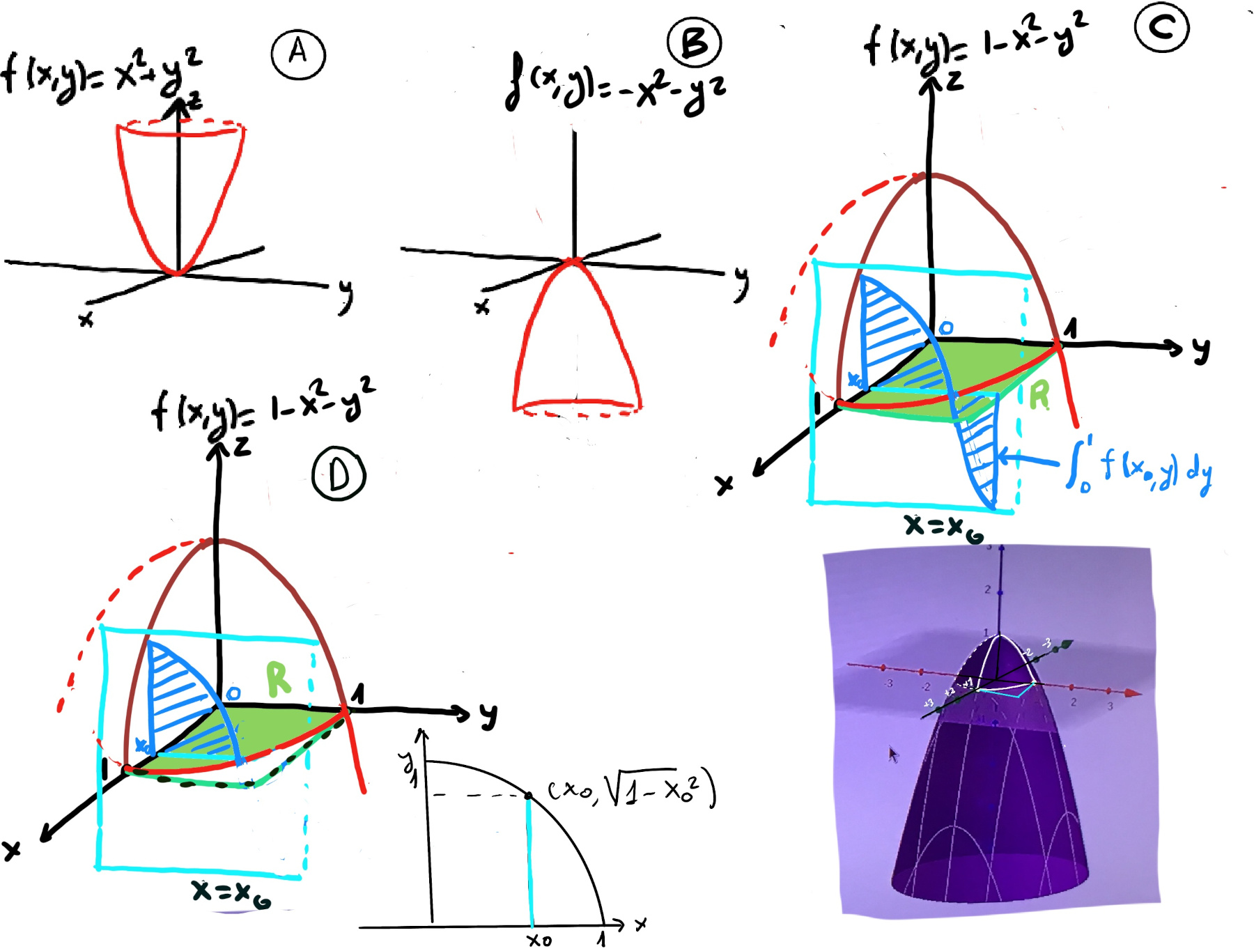
$\iint_R f(x, y) dA\ = \int_{0}^{1}(\int_{0}^{1} 1-x^2-y^2dy)dx =$[🚀]

$\int_{0}^{1} (1-x^2-y^2)dy = y -x^2y -\frac{y^3}{3}\bigg|_{0}^{1} = 1 -x^2 -\frac{1}{3} = \frac{2}{3} -x^2$

=[🚀] $\int_{0}^{1} (\frac{2}{3} -x^2)dx = \frac{2}{3}x - \frac{1^3}{3}x^3\bigg|_{0}^{1} = \frac{2}{3} - \frac{1}{3} - 0 + 0 = \frac{1}{3}$

• Let z = f(x, y) = 1 -x² -y² and the region is not going to be determined by 0 ≤ x ≤ 1, 0 ≤ y ≤ 1, but by the region between the paraboloid and the xy plane, that is, looking at the part of the paraboloid that sits above the xy plane.

Therefore, R (figure D) is a quarter disk where x²+ y² ≤ 1, x ≥ 0, and y ≥ 0

$\iint_R f(x, y) dA\ = \int_{0}^{1}(\int_{0}^{\sqrt{1-x^2}} 1-x^2-y^2dy)dx =$[🚀]

$\int_{0}^{\sqrt{1-x^2}} 1-x^2-y^2dy = (y-x^2y-\frac{y^3}{3})\bigg|_{0}^{\sqrt{1-x^2}} = \sqrt{1-x^2}-x^2\sqrt{1-x^2}-\frac{1}{3}(1-x^2)^{\frac{3}{2}}=(1-x^2)\sqrt{1-x^2}-\frac{1}{3}(1-x^2)^{\frac{3}{2}} = (1-x^2)\sqrt{1-x^2}-\frac{1}{3}(1-x^2)^{\frac{3}{2}} = (1-x^2)\sqrt{1-x^2}-\frac{1}{3}(1-x^2)^{\frac{3}{2}} = (1-x^2)^{\frac{3}{2}}-\frac{1}{3}(1-x^2)^{\frac{3}{2}} = \frac{2}{3}(1-x^2)^{\frac{3}{2}}$

=[🚀] $\int_{0}^{1} \frac{2}{3}(1-x^2)^{\frac{3}{2}}dx =$[x = sin(θ), $(1-x^2)^{\frac{1}{2}} = cos(θ)$, dx = cos(θ)dθ] $\int_{0}^{\frac{π}{2}} \frac{2}{3}cos^4(θ)dθ =[cos^2(θ)=\frac{1+cos(2θ)}{2}] = \frac{2}{3}\int_{0}^{\frac{π}{2}}(\frac{1+cos(2θ)}{2})^2dθ =\frac{2}{3}\int_{0}^{\frac{π}{2}} (\frac{1}{4}+\frac{1}{2}cos(2θ)+\frac{1}{4}cos^2(2θ))dθ=[cos^2(θ)=\frac{1+cos(2θ)}{2}] = ··· = \frac{π}{8}$

Exchanging order of integration

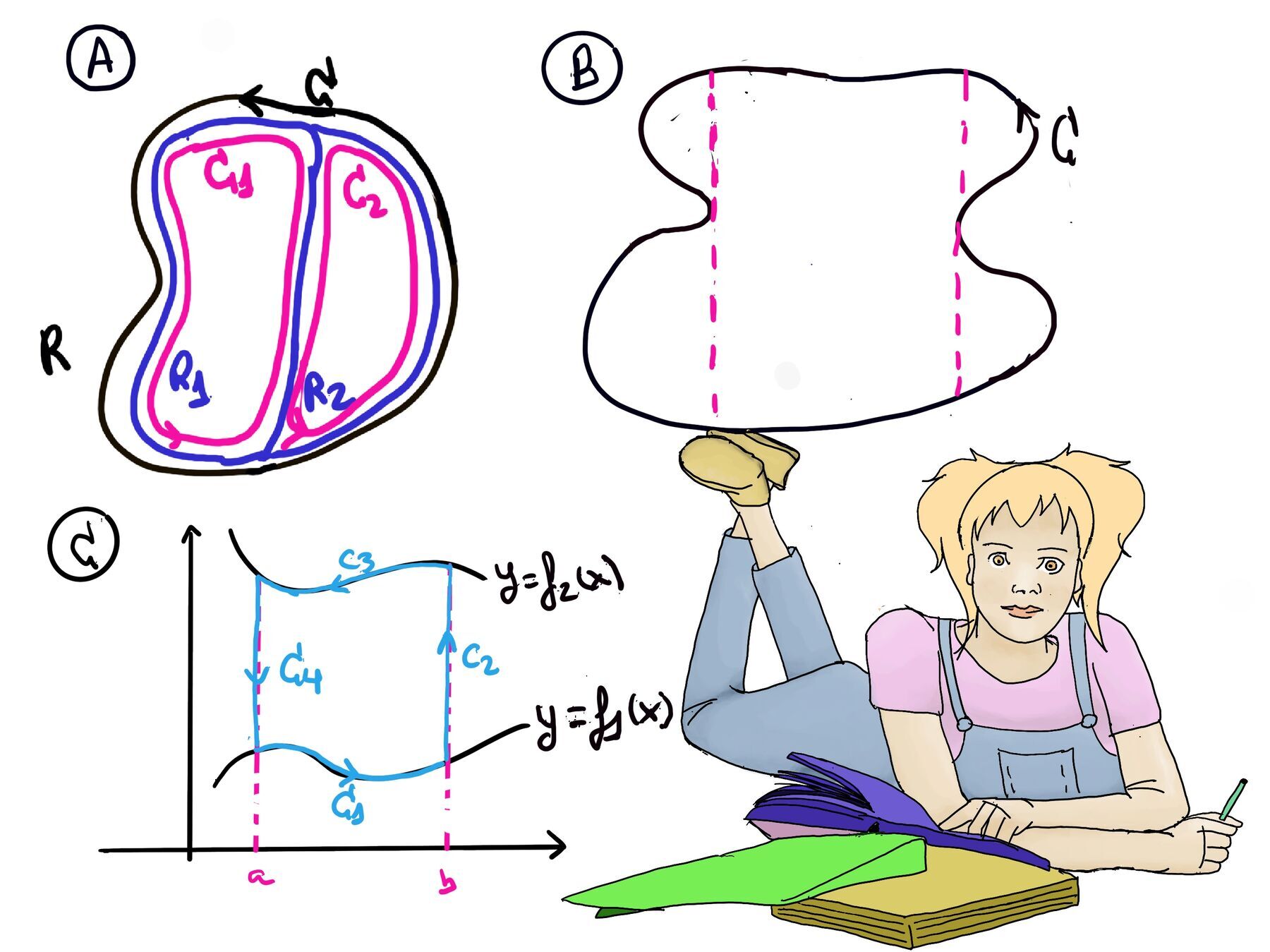
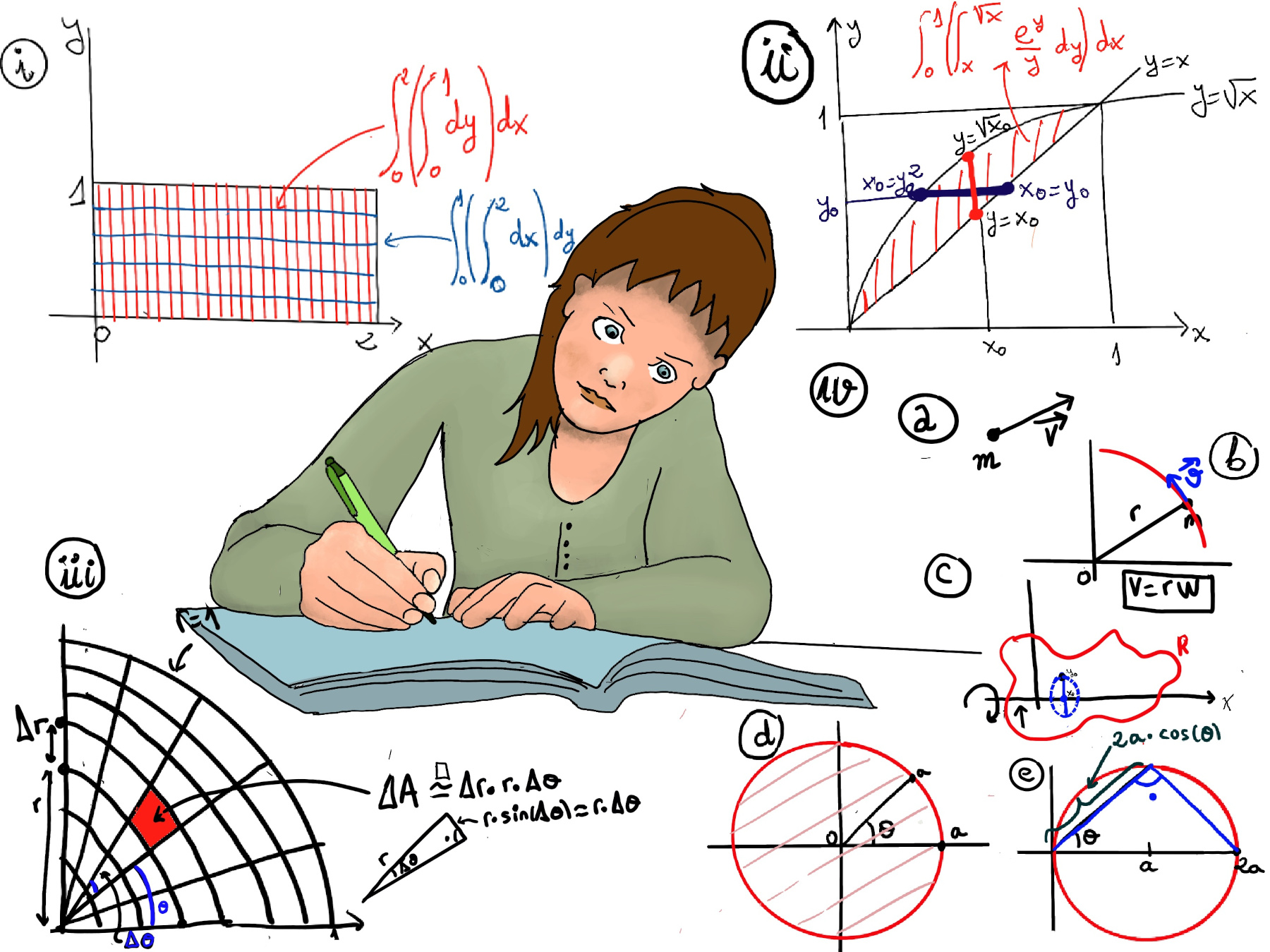
When evaluating a double integral over a region, the order of integration refers to the sequence in which we perform integration with respect to different variables, e.g., $\int_{0}^{1} (\int_{0}^{2} dx)dy = \int_{0}^{2} (\int_{0}^{1} dy)dx$ (Figure i).

This method allows us to simplify calculations by choosing the most convenient order of integration based on the given problem.

The reader should realize that the following integral $\int_{0}^{1} (\int_{x}^{\sqrt{x}} \frac{e^y}{y}dy)dx$, in its actual form is impossible to compute. We are going to exchange the order, but this will normally affect the bounds of the integrals (Figure ii) and it is not necessarily easy to see, $\int_{0}^{1} (\int_{x}^{\sqrt{x}} \frac{e^y}{y}dy)dx = \int_{0}^{1} (\int_{y^2}^{y} \frac{e^y}{y}dx)dy$.

$\int_{y^2}^{y} \frac{e^y}{y}dx = \frac{e^y}{y}x\bigg|_{y^2}^{y}=e^y-e^yy$

$\int_{0}^{1} (\int_{x}^{\sqrt{x}} \frac{e^y}{y}dy)dx = \int_{0}^{1} (\int_{y^2}^{y} \frac{e^y}{y}dx)dy = \int_{0}^{1} (e^y-e^yy)dy =$[Integration by parts the second part of the integrand, ∫udv=uv−∫vdu where u = y, dv = e^ydy, du = dy, v = e^y] $e^y-(ye^y-\int e^ydy)= 2e^y -ye^y\bigg|_{0}^{1} = 2e-e-2=e-2.$

Double integrals in polar coordinates

In double or even triple integrals, we can also use change of variables to make the computation more manageable. For example, in polar coordinates, we replace x and y with $r\cos \theta$ and $r \sin \theta$, respectively, and adjust the limits of integration accordingly.

Recall the previously calculated $\int \int_{x^2+y^2≤1, x, y≥0} (1-x^2-y^2)dx$ and that polar coordinates specifies the location of a point P in the plane by its distance r from the origin and the angle θ made counterclockwise between the line segment from the origin to P and the positive x-axis (Figure iii).

Notice that ΔA ≈ Δr·rΔθ, dA = rdrdθ. Recall that the sine function (sin(Δθ)) relates the angle (Δθ) to the ratio of the length of the side opposite the angle to the length of the hypotenuse in a right triangle, and when $Δ\theta$ is very close to 0, we can make an approximation: $\sin(Δ\theta) \approx Δ\theta$, hence $Δ\theta ≈ Δr·rΔ\theta, dA = rdrdθ, \int \int fdA = \int (\int f·rdr)dθ$

$\int \int_{x^2+y^2≤1, x, y≥0} (1-x^2-y^2)dx$ =[x = rcosθ, y = rsin(θ), f = 1 -x²-y² = 1 -r²] $\int_{0}^{\frac{π}{2}} (\int_{0}^{1} (1-r^2)rdr)dθ =$ [🚀]

$\int_{0}^{1} (1-r^2)rdr = \frac{r^2}{2}-\frac{r^4}{4}\bigg|_{0}^{1} = \frac{1}{2}-\frac{1}{4} = \frac{1}{4}$

= [🚀] $\int_{0}^{\frac{π}{2}} \frac{1}{4}dθ = \frac{1}{4}θ\bigg|_{0}^{\frac{π}{2}} = \frac{1}{4}·\frac{π}{2} = \frac{π}{8}$.

Bibliography

1. NPTEL-NOC IITM, Introduction to Galois Theory.
2. Algebra, Second Edition, by Michael Artin.
3. LibreTexts, Calculus and Calculus 3e (Apex). Abstract and Geometric Algebra, Abstract Algebra: Theory and Applications (Judson).
4. Field and Galois Theory, by Patrick Morandi. Springer.
5. Michael Penn, and MathMajor.
6. Contemporary Abstract Algebra, Joseph, A. Gallian.
7. YouTube’s Andrew Misseldine: Calculus. College Algebra and Abstract Algebra.
8. MIT OpenCourseWare 18.01 Single Variable Calculus, Fall 2007 and 18.02 Multivariable Calculus, Fall 2007.
9. Calculus Early Transcendentals: Differential & Multi-Variable Calculus for Social Sciences.