Jupyter Notebook: A Complete, Practical Guide

Assumption is the mother of all screw-ups, Anonymous.

Jupyter Notebook

Jupyter Notebook is an open-source web application that allows users to create and share documents containing live code, visualizations, mathematical equations, and narrative text. It is a powerful and widely used tool for data analysis, machine learning, scientific computing, and education due to its interactive and flexible nature.

Its key features include:

• Interactive Code Execution: Run and execute code snippets in cells, which can be run individually or in batches and see results immediately.
• Rich Text Editing and Media: You can add text, headings, lists, tables, and embed images/HTML in Markdown cells.
• Mathematical Equations: Jupyter Notebook supports LaTeX equations, allowing you to create complex mathematical expressions.

    $e^{i\pi}+1=0$
    $$\sum_{k=0}^{\infty}\frac{z^k}{k!}=e^z$$

Output: $e^{i\pi}+1=0$

• Reproducibility: Combine code, text, data, and results in a single .ipynb file.
• Visualizations: You can plot and create interactive visualizations using popular libraries like Matplotlib, Seaborn, and Plotly.
• Extensibility: You can use third-party libraries (e.g., NumPy, Pandas, Matplotlib) and tools (e.g., Git, Docker).
• Sharing, exporting, and Collaboration: Notebooks can be shared with others via URL, exported or downloaded as PDF, HTML, or IPYNB files.

  jupyter nbconvert ‐‐to html your_notebook.ipynb

Notebook vs. Lab: The classic app is Jupyter Notebook (jupyter notebook). The more modern UI is JupyterLab (jupyter lab); everything here works in both unless noted.

Installing Jupyter Notebook

Install Jupyter Notebook using pip (pip install notebook or python -m pip install notebook) or conda (conda install -c conda-forge notebook). After installation, start the notebook server by running jupyter notebook in the terminal. This command starts a web server from a terminal in your project folder and opens your browser to http://localhost:8888. Stop the server with Ctrl + C in the terminal.

Starting and Navigating Jupyter Notebook**

1. Interface Overview: Dashboard (lists files in your working/current directory). Notebook Interface: Cells are the basic building blocks. They can contain code, text (Markdown), or mathematical equations (LaTeX). Menu Bar: File, Edit, View, Run, Kernel (the process that executes code: Python, R, Julia, …), etc. Toolbar: Run, Stop, Add/Delete cells, change cell type. Output: The output area displays the results of code execution, including text, images, and visualizations.

   Core shortcuts (Help, Show Keyboard Shortcuts…): A/B insert cell above/below; DD delete; M/Y: Change cell to Markdown/Code. Shift+Enter: Run cell, select next.

2. Basic Operations: Create a New Notebook: (i) Navigate to File, New, NoteBook; (ii) Select a kernel (this is the engine that executes the code in your notebook. Popular kernels include Python, R, and Julia). Cell Types: Code Cells (for writing and executing code), Markdown Cells (for text, headings, equations, etc.). Running a Cell: Press Shift + Enter to execute and move to the next cell or Ctrl + Enter to execute in-place (stay). Save NoteBook: File, Save Notebook (.ipynb files) or Ctrl + S.

   Cells execute in the order you run them within the same kernel. Kernel, Restart kernel clears memory; Run, Run All Cells re-executes top-to-bottom for reproducibility. Kernel, Interrupt Kernel to stop long-running computations.

3. Tips and Tricks: Use Markdown for Text: Use Markdown to format text in your notebook, making it easy to read and understand. Split Code into Cells: Split long code blocks into smaller cells, making it easier to debug and test individual components. Use Visualizations: Use visualizations to communicate insights and results, making your notebook more engaging and effective.
4. Managing packages in notebooks. Inside notebooks, use IPython magics so installs target the current kernel, e.g., %pip install numpy pandas matplotlib scipy sympy, %timeit x = [i for i in range(1000000)] (timing).
5. How to Properly Write Markdown in Jupyter Notebooks. (i) Change the cell from “Code” to “Markdown” (Toolbar, Select the cell type, Markdown or M); (ii) Write Markdown directly; (iii) Run the cell to render.

# Header Example
- Bullet point
- Another bullet point
[Link to Google](https://www.google.com)

Inline math: $e^{i\pi} + 1 = 0$

Display math:
$$
\sum_{k=0}^{\infty} \frac{z^k}{k!} = e^z
$$

Using Jupyter Notebook

Basic Numerical Math (Python standard library)

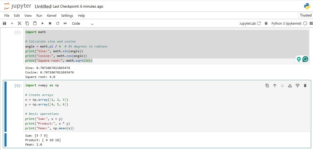
# For simple calculations, use the built-in math module in a Jupyter cell.
import math

# Calculate sine and cosine
angle = math.pi / 4  # 45 degrees in radians
print("Sine:", math.sin(angle))
print("Cosine:", math.cos(angle))
print("Square root:", math.sqrt(16))

Output:

Sine: 0.7071067811865476
Cosine: 0.7071067811865476
Square root: 4.0

import math

# Trigonometric and exponential functions
angle_deg = 60
angle_rad = math.radians(angle_deg)
print("Tan(60°):", math.tan(angle_rad))
print("e^2:", math.exp(2))
print("Log10(100):", math.log10(100))

# Constants
print("Pi:", math.pi)
print("e:", math.e)

Output:

Tan(60°): 1.7320508075688767
e^2: 7.38905609893065
Log10(100): 2.0
Pi: 3.141592653589793
e: 2.718281828459045

Array-Based Computations with NumPy

NumPy provides efficient multi-dimensional arrays for linear algebra and statistics.

# NumPy excels in vectorized math.
# Example for creating arrays and performing element-wise operations:
import numpy as np

# Create arrays
x = np.array([1, 2, 3])
y = np.array([4, 5, 6])

# Basic operations
print("Sum:", x + y)
print("Product:", x * y)
print("Mean:", np.mean(x))
print("Standard deviation: ", np.std(x))
print("Variance: ", np.var(x))

Output:

Sum: [5 7 9]
Product: [4 10 18]
Mean: 2.0
Standard deviation:  0.816496580927726
Variance:  0.6666666666666666

Advanced Scientific Math with SciPy

SciPy is like NumPy’s brainy older sibling —it takes the powerful array-handling capabilities of NumPy and layers on a rich set of scientific and technical computing tools.

SciPy handles correlations and regressions. The Pearson correlation coefficient, often denoted as r, is a statistical measure that quantifies the strength and direction of a linear relationship between two continuous variables.

Mathematically, it’s defined as: r = $\frac{\text{Cov}(X, Y)}{\sigma_X \sigma_Y}$ where:

• $\text{Cov}(X, Y)$ is the covariance between variables X and Y
• $\sigma_X$ and $\sigma_Y$ are the standard deviations of X and Y

Interpretation: r = 1, perfect positive linear correlation; r = -1, perfect negative linear correlation; r = 0, no linear correlation; 0 < r < 1, positive correlation (weak to strong); -1 < r < 0, negative correlation (weak to strong).

import numpy as np
from scipy.stats import pearsonr

x = np.arange(10, 20)
y = np.array([2, 1, 4, 5, 8, 12, 18, 25, 96, 48])
r, p = pearsonr(x, y)
print("Correlation coefficient:", r)
print("P-value:", p)

Output:

Correlation coefficient: 0.758640289091187
P-value: 0.010964341301680816

Linear regression. It’s a method for finding the straight line that best fits a set of data points. The idea is to model the relationship between two variables, x and y, using an equation:y = m x + b where m is the slope (the rate of change between x and y) and b is the intercept (where the line crosses the y-axis).

If you plot all your (x, y) data on a graph, the line won’t go through every point perfectly. Each point has a residual — the vertical distance between the actual y and the pred6icted $\hat{y}$ from the line. Least squares says: Find the line where the sum of the squares of all these residuals is as small as possible.

# Import the linregress function from the scipy.stats module
from scipy.stats import linregress
import numpy as np

# Create an array of x values ranging from 10 to 19
x = np.arange(10, 20)

# Create an array of y values for corresponding x values
y = np.array([2, 1, 4, 5, 8, 12, 18, 25, 96, 48])

# Perform linear regression on the x and y data
# linregress(x, y) computes a linear least-squares regression for the given x and y data.
# It returns the slope, intercept, correlation coefficient (r), p-value, and standard error of the estimate (se).
# p-value is the Significance test: low values suggest the relationship is unlikely due to random chance.
slope, intercept, r, p, se = linregress(x, y)

# Print the slope and intercept of the regression line
print("Slope:", slope, "Intercept:", intercept)
print("r:", r, "p-value:", p, "stderr:", se)

Output:

Slope: 7.4363636363636365 Intercept: -85.92727272727274
r: 0.7586402890911869 p-value: 0.010964341301680825 stderr: 2.257878767543913

Symbolic Math with SymPy

For exact algebraic manipulation, SymPy is a Python library for symbolic mathematics. It aims to become a full-featured computer algebra system (CAS) while keeping the code as simple as possible in order to be comprehensible and easily extensible.

# Example calculating Pearson correlation:
from sympy import symbols, solve
x = symbols('x')
# Solve a polynomial:
solution = solve(x**2 - 4, x)
print(solution)  # [-2, 2]

from sympy import symbols, diff, integrate, limit, sin

x = symbols('x')
# Calculus:
f = x**3 + 2*x**2 - 5*x
print("Derivative:", diff(f, x))
print("Integral:", integrate(f, x))

# Limits
print("Limit as x->0 of sin(x)/x:", limit(sin(x)/x, x, 0))

Output:

Derivative: 3*x**2 + 4*x - 5
Integral: x**4/4 + 2*x**3/3 - 5*x**2/2
Limit as x->0 of sin(x)/x: 1

# Solving systems:
from sympy import symbols, Eq, solve

x, y = symbols('x y')
eq1 = Eq(x + y, 5)
eq2 = Eq(x - y, 1)
solutions = solve([eq1, eq2], [x, y])
print("Solutions:", solutions)

Output: Solutions: {x: 3, y: 2}

# Numerical integration with SciPy
from scipy.integrate import quad

def integrand(x):
    return sin(x)

result, error = quad(integrand, 0, 1)
print("Integral of sin(x) from 0 to 1:", result)

Output: Integral of sin(x) from 0 to 1: 0.45969769413186023

Data Visualization

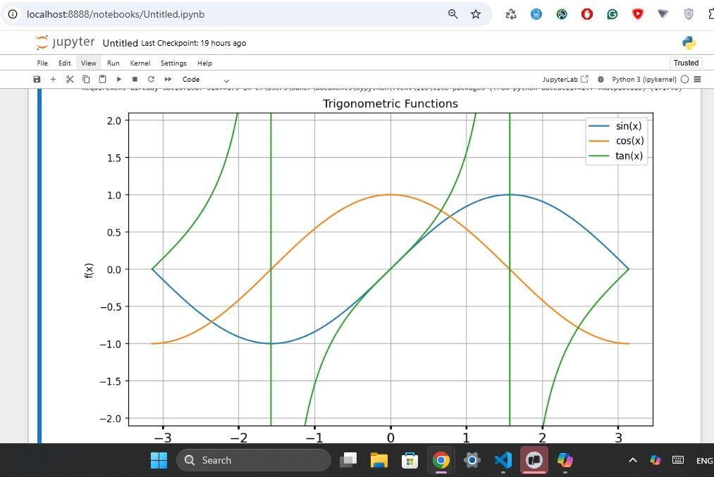
# Install the matplotlib library for plotting
!pip install matplotlib

# Import necessary libraries
import numpy as np # For numerical operations
import matplotlib.pyplot as plt # For plotting

# Create an array of 1000 points evenly spaced between -π and π
x = np.linspace(-np.pi, np.pi, 1000)

# Set up the figure size and resolution
plt.figure(figsize=(10, 6), dpi=120)

# Plot the sine, cosine, and tangent function
plt.plot(x, np.sin(x), label='sin(x)')
plt.plot(x, np.cos(x), label='cos(x)')
plt.plot(x, np.tan(x), label='tan(x)')

# Set the y-axis limits to avoid displaying tangent spikes
plt.ylim(-2.1, 2.1)

# Display the legend to identify the functions
plt.legend()
# Set the title of the plot
plt.title("Trigonometric Functions")
# Label the x-axis
plt.xlabel("x")
# Label the y-axis
plt.ylabel("f(x)")
# Enable grid lines on the plot for better readability
plt.grid(True)
# Customize tick parameters for the x-axis
plt.tick_params(axis='x', labelsize=14, width=2)
# Show the plot
plt.show()

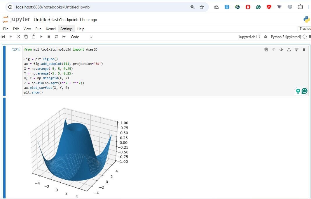
This code generates a 3D surface plot of the function $z = sin(\sqrt{x^2+y^2})$

# Import the necessary libraries for 3D plotting
import numpy as np
import matplotlib.pyplot as plt
from mpl_toolkits.mplot3d import Axes3D

# Create a new figure for the 3D plot
fig = plt.figure()

# Add a 3D subplot to the figure
ax = fig.add_subplot(111, projection='3d')

# Create a range of values for X and Y axes
X = np.arange(-5, 5, 0.25)
Y = np.arange(-5, 5, 0.25)

# Create a meshgrid for X and Y values
X, Y = np.meshgrid(X, Y)

# Calculate Z values as a function of X and Y
Z = np.sin(np.sqrt(X**2 + Y**2))

# Plot the surface of the 3D graph
ax.plot_surface(X, Y, Z, cmap='viridis')  # Adding a colormap for better visualization

# Display the plot
plt.show()

Load and Visualize Data with pandas

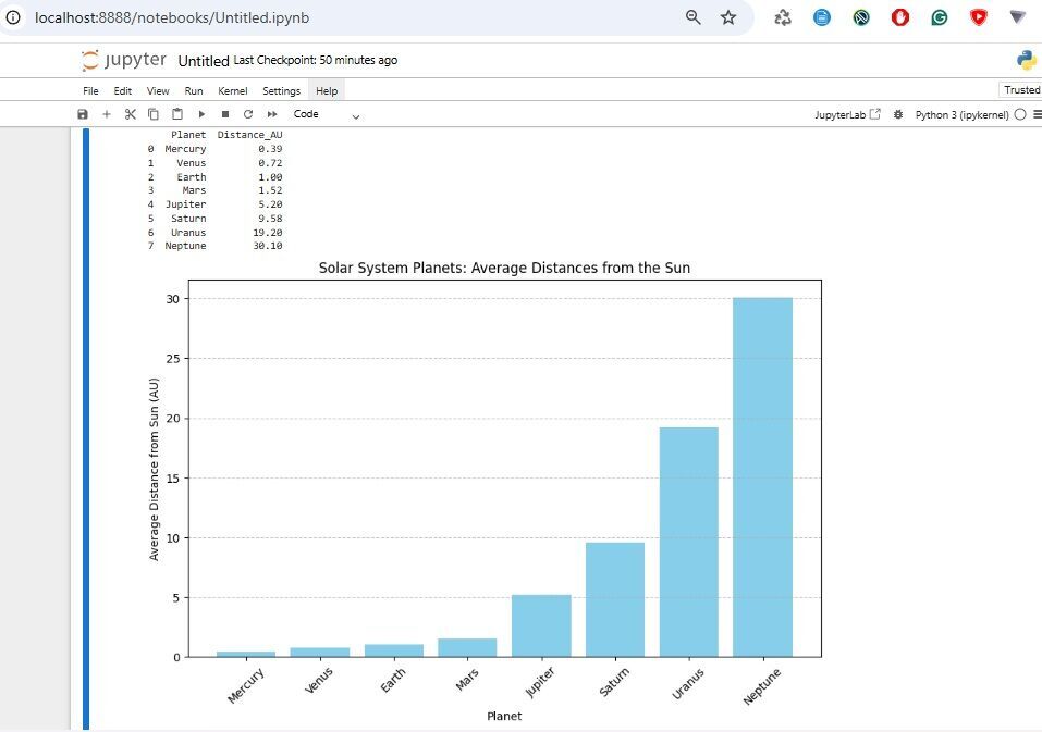
# Import the pandas library for data manipulation and matplotlib for plotting
import pandas as pd
import matplotlib.pyplot as plt

# Create a dictionary containing planet names and their average distances from the Sun in astronomical units (AU)
data = {
    'Planet': ['Mercury', 'Venus', 'Earth', 'Mars', 'Jupiter', 'Saturn', 'Uranus', 'Neptune'],
    'Distance_AU': [0.39, 0.72, 1.00, 1.52, 5.20, 9.58, 19.20, 30.10]
}

# Convert the dictionary into a pandas DataFrame for easier data manipulation
df = pd.DataFrame(data)

# Print the DataFrame to the console
print(df)

# Set up the figure size for better readability
plt.figure(figsize=(10, 6))

# Create a bar chart using the DataFrame data
plt.bar(df['Planet'], df['Distance_AU'], color='skyblue')

# Label the x-axis for clarity
plt.xlabel('Planet')

# Label the y-axis for clarity
plt.ylabel('Average Distance from Sun (AU)')

# Set the title of the plot
plt.title('Solar System Planets: Average Distances from the Sun')

# Rotate x-axis labels for better visibility
plt.xticks(rotation=45)

# Add a grid line along the y-axis for better readability of values
plt.grid(axis='y', linestyle='--', alpha=0.7)

# Display the plot
plt.show()

Reproducibility, Best practices, and troubleshooting

1. Use a clean kernel: Restart & Run All before sharing to ensure a clean, linear run.
2. Pin package versions (e.g., requirements.txt or environment.yml).
3. Keep notebooks light: avoid huge outputs; save figures/data to files. Save often.
4. Treat downloaded notebooks as untrusted: don’t run unknown code, review before running.
5. Consider factoring reusable code into modules and importing them.
6. Module not found: Ensure you installed the package into the same environment as the kernel (if needed, reinstall with %pip install package-name).
7. Use Markdown generously to explain context, assumptions, and results.
8. Kernel busy forever: Try Kernel, Interrupt Kernel; if stuck, Kernel, Restart Kernel.
9. Plots not showing: Add %matplotlib inline (classic Notebook) or ensure the cell finishes executing and call plt.show().
10. Math not rendering: Put LaTeX in a Markdown cell (not a code cell) and use $···$ or $$···$$.