Types of functions

My appearance had improved substantially, but my pictures could still be sold to scare people, summon the devil, and kill the elderly. I was notice immediately, so many of my coworkers felt embarrassed and avoid hanging with me like eating shit or alien foreskin, Apocalypse, Anawim, #justtothepoint.

Recall

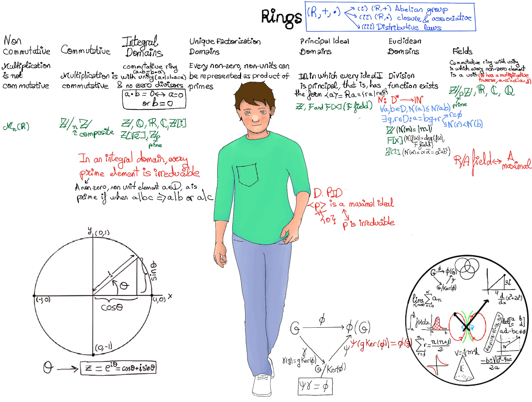
Definition. A function f is a rule, relationship, or correspondence that assigns to each element x in a set D, x ∈ D (called the domain) exactly one element y in a set E, y ∈ E (called the codomain or range).

• The pair (x, y) is denoted as y = f(x) where: x is the independent variable (input) and y is the dependent variable (output). Often, both the domain D and codomain E are the set of real numbers ℝ or subsets of ℝ. A mathematical function can be thought of as a black box (or machine) that takes an input from its domain and produces exactly one output in its codomain. Inside the machine lives a specific rule (formula, procedure, or mapping) that dictates or tells you which output corresponds to each input, and a key property is uniqueness —each input maps to a single, deterministic output. No input can ever produce two different results (Figure E). The function f(x) = x² accepts any real number x (domain: ℝ) and returns exactly one non-negative value x² (output in codomain: [0,∞)). The input 3 always yields 9, never any other value.

• D is the domain, the set of all possible inputs. E is the codomain or range, the set of all possible outputs.

• Key property💡: Each input has exactly one output. (No input is assigned two different outputs — this is the vertical line test!)

• Examples: constant, f(x) = c, horizontal line, slope = 0; linear, f(x) = mx + b, straight line, constant slope m and y-intercept b; quadratic $f(x) = ax^2 + bx + c$, u-shaped or inverted U, opens up (a > 0) or down (a < 0), vertex at x = $\frac{-b}{2a}$, symmetry about vertical axis through vertex; polynomial, $f(x) = a_n x^n + \dots + a_0$, a smooth and continuous curve, n roots (counting multiplicity), end behaviour determined by its leading term $a_n x^n$; exponential function, $f(x) = a \cdot b^x, a \ne 0, b \gt 0$, rapid growth (b > 1) or decay (0 < b < 1); trigonometric functions, $\sin(x), \cos(x), \tan (z)$ oscillatory, periodic behavior (period 2π for sin/cos, π for tan), sin and cos are bounded between -1 and 1, but tan is unbounded; step function $f(x) = \lfloor x \rfloor$, greatest integer ≤ x, constant on intervals [n, n+1), jumps at integers, its graph is a staircase shape; absolute value f(x) = |x|, V-shaped graph, slope changes at 0.

• Functions can be expressed in multiple forms, each useful in different contexts: verbal description, table of values (list of pairs), algebraic formula, graph, piecewise definition, recursive definition, parametric or integral form, and series representation.

• Evaluating a function means finding or computing the output value f(x) for a given input value x. f(x) = $x^2-2x +4, f(2) = 2^2 -2\cdot 2 + 4 = 4 - 4 + 4 = 4, f(0) = 0^2 -2\cdot 0 + 4 = 4, f(1) = 1^2 -2\cdot 1 + 4 = 1 -2 +4 = 3$

• The x-intercept is any point on the graph that intersects or crosses the x-axis. In other words, it is the value of x when the function (y-coordinate or y-value) is zero. The y-intercept is the point where the graph intersects or crosses the y-axis. y-coordinate of the point whose x-coordinate is 0, e.g., 2x - 3y = 6. x-intercept: set y = 0 → 2x = 6 ⇒ x=3, so (3, 0). y-intercept: set x = 0 → −3y = 6 ⇒ y = −2, so (0, −2).

• f is said to have a local or relative maximum at c if there exists an interval (a, b) containing c ($c \in (a, b)$) such that f(c) ≥ f(x) $∀ x \in (a, b) ∩ D$. f is said to have a local or relative minimum at c if there exists an interval (a, b) containing c ($c \in (a, b)$) such that f(c) ≤ f(x) $∀ x \in (a, b) ∩ D$.💡Local extrema can only occur where the function stops rising or falling —either because the derivative is zero, the derivative doesn't exist, or you're at the edge of the domain.

• First Derivative Test. Let f be differentiable on an open interval containing c, except possibly at c itself, and let c be a critical point (so f′(c) = 0 or f′ is undefined). Then:

1. If f′(x) > 0 for x just to the left of c and f′(x) < 0 for x just to the right of c, then f(c) is a local maximum.
2. If f′(x) < 0 for x just to the left of c and f′(x) > 0 for x just to the right of c, then f(c) is a local minimum.
3. If f′(x) does not change sign at c (stays positive or stays negative), then f(c) is not a local extremum.

• Second Derivative Test. If the first derivate of a function at a point c is zero (f'(c) = 0) and the second derivate at this point exists, then: (i) If f''(c) > 0, then f(c) is a local minimum. (ii) If f''(c) < 0, then f(c) is a local maximum. (iii) If f''(c) = 0, the test is inconclusive.
• Vertical asymptotes are vertical lines (perpendicular to the x-axis) of the form x = a (where a is a constant) near which the function grows without bound when x approaches a from at least one side. The line x = a is a vertical asymptote of f if at least one of the one-sided limits is infinite: $\lim_{x \to a^{-}}f(x)=\pm\infty$ or $\lim_{x \to a^{+}}f(x)=\pm\infty$.
• Horizontal asymptotes are horizontal lines (y = c, parallel to the x-axis) that the graph of the function approaches as x grows very large (positively or negatively). In other words, the function values get arbitrarily close to c as long as x is sufficiently large or more formally: $\lim_{x \to \infty}f(x)=c$ and/or $\lim_{x \to -\infty}f(x)=c$.
• A line y = m+b is an oblique (slant) asymptote as $x \to \infty$ if $\lim_{x\to\infty} [f(x) - (mx+b)] = 0.$ This means that the curve of f(x) gets more and more closer to the line y = mx + b as x grows large. For an asymptote y = mx + b as $x \to \infty, m = \lim_{x\to\infty} \frac{f(x)}{x}, b = \lim_{x\to\infty} \bigl(f(x) - m x\bigr)$, provided both limits exist.

Types of functions

There are many types of functions in mathematics. There are different classifications, but some of the common ways to classify functions are based on the following criteria:

• Mapping: one-to-one or injective (different inputs give different outputs, e.g., f(x) = 2x + 1), surjective or onto (every element of the codomain is attained by some input, e.g., $f(x) = e^x$ is surjective onto (0, ∞)), and bijective (both injective and surjective. A bijection has a well-defined inverse function $f^{-1}$, e.g., $f: \mathbb{R} \to \mathbb{R}, f(x) = x^3$).

• Symmetry and periodicity: even (f(x)=f(-x), it has symmetry with respect to the y-axis, e.g., |x|, x², cos(x)), odd (f(-x)=-f(x), it has rotational symmetry with respect to the origin, that is, its graph remains unchanged after rotation of 180° about the origin, e.g., sgn(x), x, x³, sin(x)), periodic (it has a graph with a basic pattern that repeats at regular intervals, there exists T > 0 with f(x) = f(x + T) for all x, e.g., sin(x) and cos(x) are periodic with period T = 2π).

• Functions are grouped by how smooth they are, ranging from highly irregular (discontinuous) to perfectly smooth, i.e., analytic. Discontinuous functions are characterized by having breaks or jumps in their graphs, e.g., the Dirichlet function is nowhere continuous, $f(x) = \begin{cases} 1, &x \in \mathbb{Q} \\\\ 0, &x \in \mathbb{R} \setminus \mathbb{Q} \end{cases}$ and step functions, piecewise functions that outputs a constant value over different intervals, creating a graph of horizontal segments resembling steps (such as the Greatest Integer Function or floor function, [x], which gives the largest integer less than or equal to x, and the Heaviside Step Function, which is zero for negative inputs and one for positive inputs). Continuous functions: no jumps or holes, limit matches value at every point $\lim_{x \to a}f(x) = f(a)$. Differentiable: Derivative exists everywhere. $C^1$: Derivative exists and is continuous, $C^k$: k-times continuously differentiable, and $C^\infty$ infinitely differentiable (smooth). A function is analytic if and only if for every $x_0$ in its domain, its Taylor series about $x_0$ converges to the function in some neighborhood of $x_0$, e.g., polynomials, $, \sin(x), \cos(x), e^x$

• Functions are also classified by how rapidly their values grow and whether they remain within finite bounds. Bounded (f(x) stays within some finite range, e.g., $\sin(x), \cos(x)$ are bounded between [-1, 1]) and Unbounded (they can become arbitrarily large, e.g. polynomials of odd degree $x, x^3$, rational functions near vertical asymptotes $\frac{1}{x-a}$). Growth Rate Hierarchy: Constant (e.g, 5, 7, O(1), lowest); Logarithmic (ln(x), O(lnx)); Sublinear ($\sqrt{x}$, o(x)); Linear (x, O(x)); Polynomial ($x^2, x^3, O(x^k)$); Exponential ($e^x, 2^x, O(a^x)$); Factorial (x!, O(x!), fastest).

• Functions are classified by whether they are invertible and how their values change (monotonicity). Increasing: f(x₁​) ≤ f(x₂​) for x₁ < x₂; Strictly increasing: f(x₁)< f(x₂) for x₁ < x₂; Decreasing: f(x₁) ≥ f(x₂) for x₁ < x₂; Strictly decreasing: f(x₁) > f(x₂) for x₁ < x₂; Monotone: Either increasing or decreasing. Strict monotonicity on an interval guarantees injectivity and invertibility onto the function’s range, $f^{-1}: f(I)\rightarrow I$. Derivative Test for Monotonicity: If f′(x) > 0, f is strictly increasing there. If f′(x) < 0, f is strictly decreasing. If f′(x) ≥ 0, f is non-decreasing (but not necessarily strictly).

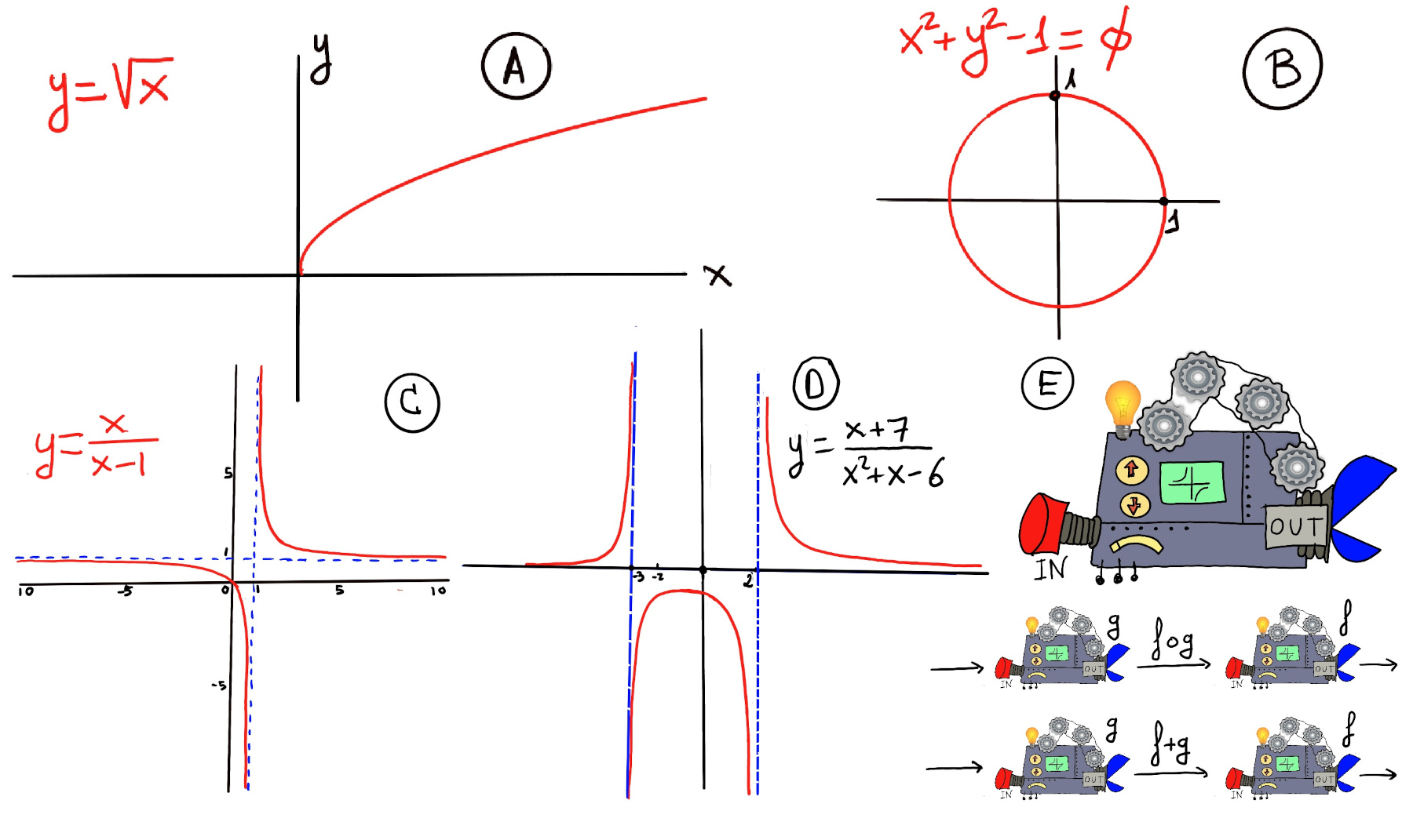
• Implicit & parametric functions. An implicit function is defined by a relation involving two or more variables, typically of the form F(x, y) = 0, rather than by an explicit formula for one variable in terms of another, e.g., the circle: $x^2+y^2=r^2$ defines y implicitly as a function of x; or the sphere, $x^2+y^2+z^2=1$. In the circle, solving for y gives two explicit branches: $y = \pm \sqrt{r^2-x^2}$ but the original relation is implicit and often more natural for describing geometric objects. Implicit Differentiation: Used to find derivatives when y is not isolated, e.g., $x^4+2y^2=8 \implies 4x^3+4y\frac{dy}{dx}=0 \implies \frac{dy}{dx} = \frac{-x^3}{y}$. A parametric function expresses each coordinate as a function of one or more independent parameters. In 2D, x = f(t), y = g(t) where t is the parameter. In 3D, x = f(t), y = g(t), z = h(t). Parametric forms can describe curves and surfaces that are difficult or impossible to represent as explicit functions. Examples: circle ( $x = r\cos(t), y = r\sin(t), t \in [0, 2\pi)$), cycloid (the curve traced by a point on a circle as it rolls along a straight line without slipping, $x = r(t− \sin(t)), y = r(1 −\cos(t))$), sphere ($x = r\sin(\phi)\cos(\theta), y = r\sin(\phi)\sin(\theta),z = r\cos(\phi)$), helix ($x = r\cos(t), y = r\sin(t), z = ct$).

• Single‑Variable vs. Multivariable. A function $f:\mathbb{R}\rightarrow \mathbb{R}$ assigns a real number to each real input. A multivariable function is a function of two or more independent variables, e.g., f(x, y) or g(x, y, z), $f:\mathbb{R^{\mathnormal{n}}}\rightarrow \mathbb{R}$. It assigns a unique real number (output) to each n-tuple (input).

1. Domain and Range: The domain is a subset of $\mathbb{R}^n$; the range is the set of all possible outputs.
2. Level Sets: The set {(x, y) : f(x, y) = c} forms a level curve; and the set {(x, y, z) : f(x, y, z) = c} forms a level surface.
3. Partial Derivatives: $\frac{\partial f}{\partial x_i}$. Measure the rate of change with respect to one variable, holding others constant.
4. Gradient: $\nabla f=\left( \frac{\partial f}{\partial x_1},\dots ,\frac{\partial f}{\partial x_n}\right)$. The vector of all partial derivatives, pointing in the direction of steepest ascent. It is orthogonal to level sets.
5. Directional Derivatives. $D_{\mathbf{u}}f=\nabla f\cdot \mathbf{u}$. Rate of change in any direction $\mathbf{u}$.
6. Tangent Planes and Linear Approximation: At a point (a, b): $L(x, y) = f(a,b) + f_x(a,b)(x-a) +f_y(a,b)(y-b)$. Generalizes the tangent line to higher dimensions.
7. The Hessian Matrix $H_f=\left[ \frac{\partial ^2f}{\partial x_i\partial x_j}\right]$ is the definitive tool for classifying critical points in multivariable calculus. Critical points satisfy $\nabla f=0$. Let $Δ = det⁡(H) =f_{xx}f_{yy}-(f_{xy})^2$ evaluated at the critical point: (1) Δ > 0, $f_{xx} \gt 0$, local minimum, e.g., f(x, y) = $x^2 + y^2$, local minimum (0, 0). (2) Δ > 0, $f_{xx} \lt 0$, local maximum, e.g., f(x, y) = $-x^2 -y^2$, local maximum (0, 0). (3) Δ < 0, saddle point, e.g., f(x, y) = $x^2 - y^2$. (4) Δ = 0, degenerate (inconclusive)

Important named families

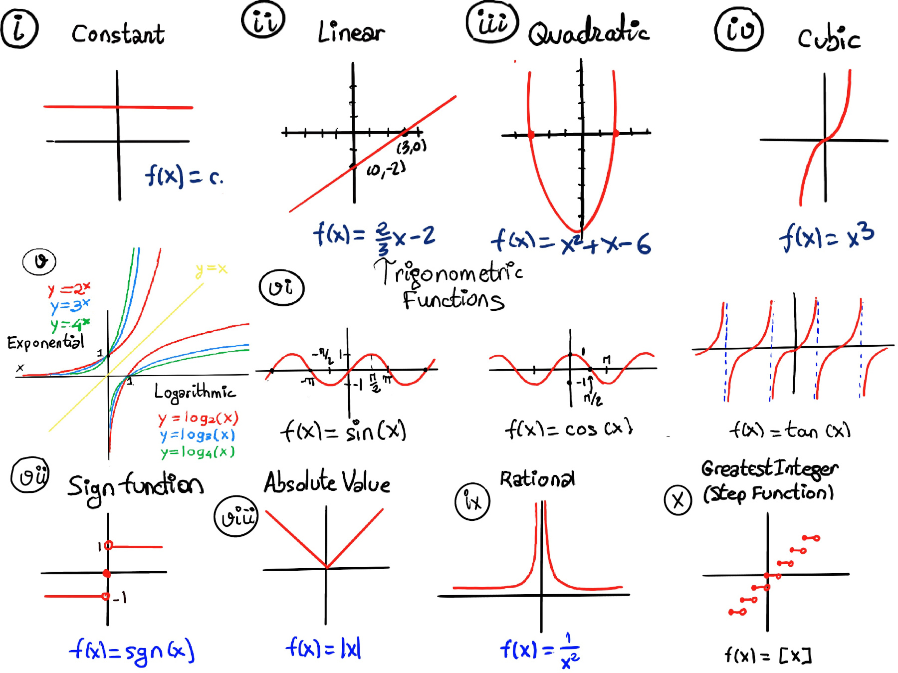
1. Linear functions. f(x) = mx + b, where m and b are constant. The graph is a straight line with a constant slope, m. m is the slope of the line (it determines the steepness or inclination of the line) and b is the y-intercept, f’(x) = m, e.g., f(x) = 2 (Figure i), f(x) = 3x -1, f(x) = 2x +7, f(x) = ²⁄₃x -2 (Figure ii).

   Algebraic functions are functions that can be expressed as a finite combination of the algebraic operations of addition, subtraction, multiplication, division, and raising to a power. Examples of algebraic functions include polynomial (f(x) = a_nxⁿ + a_n-1x^n-1 +···+ a₁x + a₀) and rational functions.

2. Quadratic Functions. A quadratic function is a polynomial with a degree of 2, f(x) =ax² + bx +c, where a, b and c are constants and a ≠ 0. The graph is a parabola with a U-shaped curve. If a > 0, then the parabola opens up “U” (minimum at vertex). If a < 0, then the parabola opens down “∩” (maximum at vertex). The vertex is the lowest or highest point on the graph, ($\frac{-b}{2a}, f(\frac{-b}{2a})$), e.g., x²+x -6, its roots are x = -3 and 2, and its vertex is ($\frac{-1}{2}, \frac{-25}{4}$) (Figure iii).

   The roots or zeros of the function are the values of x that make the function equal to zero and you can calculate them by using the quadratic formula, $\frac{-b±\sqrt{b^2-4ac}}{2a}$. Besides, the discriminant, which is the expression b² - 4ac, is used to determine the number and type of roots. If the discriminant is positive, the function has two distinct real roots and the parabola crosses the x-axis at two different points. If the discriminant is zero, the function has one repeated real root and the parabola touches the x-axis at exactly one point (the vertex). If the discriminant is negative, the function has two complex roots and the parabola does not intersect the x-axis.

3. Cubic functions. A cubic function is a polynomial with a degree of 3, f(x) =ax³ + bx² +cx +d, where a, b, c and d are real constants and a ≠ 0, e.g., f(x) = x³ (Figure iv), f(x) = 4x³ +7x² -5. An inflection point occurs when the second derivative f″(x) = 6ax + 2b is zero, and the third derivative is nonzero. Thus a cubic function has always a single inflection point, which occurs at $x_{\text{inflection}}=-\frac{b}{3a}, f'''(x)=6a \ne 0$ (since $a \ne 0$).

4. Exponential functions. An exponential function is a mathematical function of the form f(x) = b·a^x, where the independent variable is the exponent, and a and b are constants. a is called the base of the function and is a positive real number (a > 0) (Figure v). If a > 1, f is increasing; if 0 < a < 1, f is decreasing. The derivative of $f(x) = a^x$ with respect to x is given by: $\frac{d}{dx} a^x = a^x \ln(a)$. In the special case where the base is the Euler’s number ($e \approx 2.718$), the derivative simplifies to: $\frac{d}{dx} e^x = e^x$. This means the exponential function $e^x$ is unique in that its rate of change at any point equals its value at that point.

   Transcendental functions are those that are not algebraic, including exponential, trigonometric, and logarithmic functions.

5. Logarithmic functions. The logarithm is the inverse function of exponentiation. We call the inverse of a^x the logarithmic function with base a, that is, log_ax=y ↔ a^y=x, that means that the logarithm of a number x to the base a is the exponent y to which a must be raised to yield or produce x, (Figure v). The domain of logarithmic functions is $(0, \infty)$. This means that logarithms are only defined for positive real numbers. The range of logarithmic functions is all real numbers. The derivative of the logarithmic function is given by: $\frac{d}{dx} \log_a(x) = \frac{1}{x \ln(a)}$. The natural logarithm, denoted as $\ln(x)$, is a specific logarithmic function where the base a is Euler’s number e (approximately 2.71828). It is the most commonly used logarithmic function in mathematics, science, and engineering.​ Some important identities include: $\log_a(a) = 1, \log_a(1) = 0, log_a(a^x) = x, \log_a(b) = \frac{\log_c(b)}{\log_c(a)}$ (changer of base formula for any positive base c).

6. Trigonometric functions are essential mathematical functions that relate angles to the ratios of the sides of right triangles (Figure vi). They are widely used in fields such as calculus, physics, engineering, and computer science, particularly in scenarios involving angles and distances. There are six primary trigonometric functions, which are: (i) Sine: The ratio of the length of the opposite side to the hypotenuse; (ii) Cosine: The ratio of the length of the adjacent side to the hypotenuse; (iii) Tangent: The ratio of the length of the opposite side to the adjacent side. (iv) Cosecant: The reciprocal of sine, defined as $\csc(\theta) = \frac{1}{\sin(\theta)}$; (v) Secant: The reciprocal of cosine, defined as $\sec(\theta) = \frac{1}{\cos(\theta)}$; (vi) Cotangent: The reciprocal of tangent, defined as $cot(\theta) = \frac{1}{\tan(\theta)}$.

   Trigonometric functions are periodic, meaning they repeat their values at regular intervals; e.g., the sine and cosine functions have a period of $2\pi$ radians, which means that $\sin(\theta + 2\pi) = \sin(\theta), \cos(\theta + 2\pi) = \cos(\theta)$.

    

7. Piecewise functions are mathematical functions that are defined by different expressions based on the input value x. These functions allow for varying behaviors across different intervals of their domain. A piecewise function is typically expressed in the following format: $f(x)= \begin{cases} \text{expression 1}, & \text{if condition 1} \\\\ \text{expression 2}, & \text{if condition 2} \\\\ \text{expression 3}, & \text{if condition 3} \end{cases}$.

   The absolute value function can be defined as: $f(x) = \begin{cases} x, &x ≥ 0 \\\\ -x, &x < 0 \end{cases}$

   This function returns the non-negative value of x, effectively measuring the distance from zero on a number line (Figure viii).

   The sign function, which indicates the sign of a real number, can be defined as: $f(x) = \begin{cases} -1, &x < 0 \\\\ 0, &x = 0 \\\\ 1, &x > 0 \end{cases}$

   This function returns -1 for negative numbers, 0 for zero, and 1 for positive numbers (Figure vii).

8. Rational functions are defined as functions that can be expressed as the ratio of two polynomial functions. Specifically, a rational function f(x) can be written in the form: $f(x) = \frac{P(x)}{Q(x)}$ where P(x) and Q(x) are both polynomials, and importantly, $Q(x) \neq 0$. This means that the denominator cannot be zero, as this would make the function undefined, e.g., f(x) = $\frac{1}{x^2}$ (it is not defined at x = 0, Figure ix)-, $f(x)=\frac{x^2-5}{x^2+2}$. Rational functions can exhibit vertical and horizontal asymptotes. Vertical asymptotes occur at the values of x that make the denominator zero, while horizontal asymptotes describe the behavior of the function as x approaches infinity.

9. A step function, also known as a staircase function, is a type of piecewise constant function characterized by a finite number of constant values over specified intervals. It changes its value only at distinct points, creating a “step-like” appearance when graphed. Formally, a step function is defined as follows: $f(x) = \begin{cases} c_1 & \text{if } a_1 \leq x < a_2 \\\\ c_2 & \text{if } a_2 \leq x < a_3 \\\\ \vdots \\\\ c_n & \text{if } a_n \leq x < a_{n+1} \end{cases}$

   One of the most commonly used step functions is the greatest integer function, also known as the floor function, denoted as ⌊x⌋. This function returns the largest integer less than or equal to x, ⌊x⌋ = floor(x) = max{n ∈ ℤ: n ≤ x}, e.g., ⌊2.8⌋ = 2, ⌊4.3⌋ = 4, ⌊-2.3⌋ = -3. The greatest integer function is discontinuous at integer values, where it jumps from one integer to the next.

10. Power and radical functions. Power functions have the form f(x) = $x^r, r\in \mathbb{R}$. The domain depends on the exponent r. For example, $x^{1/2}=\sqrt{x}$ requires $x \ge 0$. The square root function is only defined for positive numbers and its curve forms a half-parabola (figure A). Even roots (square root, fourth root) require x ≥ 0, but odd roots (cube root, fifth root) allow all real x. Radical functions are mathematical functions that include a radical expression, e.g., the square root function f(x) = $\sqrt{x}; \sqrt[3]{x-4}; \sqrt{x-4}+5$, domain: x ≥ 4, range: y ≥ 5. The domain of a radical function is determined by the requirement that the expression under the radical (radicand) must be non-negative for even roots.  

11. In mathematics, hyperbolic functions are analogues of the ordinary trigonometric functions, but defined using the hyperbola ($x^2-y^2=1$) rather than the unit circle $x^2+y^2=1$. Hyperbolic sine: the odd part of the exponential function, that is, $\sinh(x) = \frac{e^x-e^{-x}}{2}$. Hyperbolic cosine: the even part of the exponential function, that is,​ $\cosh(x) = \frac{e^x+e^{-x}}{2}$. Hyperbolic tangent: $\tanh(x) = \frac{\sinh(x)}{\cosh(x)}=\frac{e^x-e^{-x}}{e^x+e^{-x}}$. Hyperbolic Cotangent, $x\ne 0, \coth(x) = \frac{\cosh(x)}{\sinh(x)} = \frac{e^x+e^{-x}}{e^x-e^{-x}}$. Hyperbolic secant, $sech(x) = \frac{1}{\cosh(x)} = \frac{2}{e^x+e^{-x}}$. Hyperbolic cosecant, $x\ne 0, csch(x) = \frac{1}{\sinh(x)} = \frac{2}{e^x-e^{-x}}$. Fundamental Identity (the hyperbolic Pythagorean identity): $\cosh⁡^2(x)− \sinh^⁡{2}(x)=1$.

12. Inverse Trigonometric Functions. Trigonometric functions are periodic and therefore not one-to-one. To define inverse functions, we must restrict their domains so they could pass the Horizontal Line Test. Arcsin is the inverse of the sine function, meaning it finds the angle whose sine is a given number, taking an input between -1 and 1 and returning an angle within the range of -π/2 to π/2, e.g. arcsin(0) = 0, arcsin(1) = π/2, arcsin(-1) = -π/2. Arccos is the inverse of the cosine function used to determine the angle whose cosine is a given value. Its domain is the interval [-1, 1] and the range is the interval [0, π], e.g., arccos(0) = π/2, arccos(1)=0, arccos(-1) = π. The arctan function is the inverse of the tangent function used to determine the angle whose tangent is a specific value. Its domain is all real numbers and the range is the interval (-π/2, π/2), e.g., arctan(0) = 0, arctan(±∞) = ±π/2.

13. The Dirichlet function is defined as,

    $f(x) = \begin{cases} a, &x ∈ ℚ \\\\ b, &x ∉ ℚ \end{cases}$ (typically a = 1, b = 0). It is a classic example of a function that is discontinuous everywhere, at every point in its domain. It shows pathological behaviour.

14. Implicit functions. An implicit function is a function that is defined by an implicit equation. That means the dependent and independent variables are related through an equation, but the dependent variable is not explicitly expressed in terms of the independent variable, e.g., the circle equation x²+y² = r² (figure B), elliptical equation ($\frac{x^2}{a^2}+\frac{y^2}{b^2}-1=0$) (a standard ellipse centered at the origin with width 2a and height 2b or semi-major axis a and semi-minor axis b), y² + xy = 0, y² -4x = 0.

Bibliography

1. NPTEL-NOC IITM, Introduction to Galois Theory.
2. Algebra, Second Edition, by Michael Artin.
3. LibreTexts, Calculus. Abstract and Geometric Algebra, Abstract Algebra: Theory and Applications (Judson).
4. Field and Galois Theory, by Patrick Morandi. Springer.
5. Michael Penn, and MathMajor.
6. Contemporary Abstract Algebra, Joseph, A. Gallian.
7. YouTube’s Andrew Misseldine: Calculus. College Algebra and Abstract Algebra.
8. MIT OpenCourseWare 18.01 Single Variable Calculus, Fall 2007 and 18.02 Multivariable Calculus, Fall 2007.
9. Calculus Early Transcendentals: Differential & Multi-Variable Calculus for Social Sciences.