Graphing functions

“I hope you rot in the deepest, darkest, and filthiest pit of hell where you really belong, being tormented day and night watching adds, CNN, MSNBC, and woke movies and series forever,” Apocalypse, Anawim, #justtothepoint.

Recall

Definition. A function f is a rule, relationship, or correspondence that assigns to each element x in a set D, x ∈ D (called the domain) exactly one element y in a set E, y ∈ E (called the codomain or range).

• The pair (x, y) is denoted as y = f(x) where: x is the independent variable (input) and y is the dependent variable (output). Often, both the domain D and codomain E are the set of real numbers ℝ or subsets of ℝ.

• D is the domain, the set of all possible inputs. E is the codomain or range, the set of all possible outputs.

• Key property💡: Each input has exactly one output. (No input is assigned two different outputs — this is the vertical line test!)

• Examples: constant, f(x) = c, horizontal line, slope = 0; linear, f(x) = mx + b, straight line, constant slope m and y-intercept b; quadratic $f(x) = ax^2 + bx + c$, u-shaped or inverted U, opens up (a > 0) or down (a < 0), vertex at x = $\frac{-b}{2a}$, symmetry about vertical axis through vertex; polynomial, $f(x) = a_n x^n + \dots + a_0$, a smooth and continuous curve, n roots (counting multiplicity), end behaviour determined by its leading term $a_n x^n$; exponential function, $f(x) = a \cdot b^x, a \ne 0, b \gt 0$, rapid growth (b > 1) or decay (0 < b < 1); trigonometric functions, $\sin(x), \cos(x), \tan (z)$ oscillatory, periodic behavior (period 2π for sin/cos, π for tan), sin and cos are bounded between -1 and 1, but tan is unbounded; step function $f(x) = \lfloor x \rfloor$, greatest integer ≤ x, constant on intervals [n, n+1), jumps at integers, its graph is a staircase shape; absolute value f(x) = |x|, V-shaped graph, slope changes at 0.

• Functions can be expressed in multiple forms, each useful in different contexts: verbal description, table of values (list of pairs), algebraic formula, graph, piecewise definition, recursive definition, parametric or integral form, and series representation.

• Evaluating a function means finding or computing the output value f(x) for a given input value x. f(x) = $x^2-2x +4, f(2) = 2^2 -2\cdot 2 + 4 = 4 - 4 + 4 = 4, f(0) = 0^2 -2\cdot 0 + 4 = 4, f(1) = 1^2 -2\cdot 1 + 4 = 1 -2 +4 = 3$

• The x-intercept is any point on the graph that intersects or crosses the x-axis. In other words, it is the value of x when the function (y-coordinate or y-value) is zero. The y-intercept is the point where the graph intersects or crosses the y-axis. y-coordinate of the point whose x-coordinate is 0, e.g., 2x - 3y = 6. x-intercept: set y = 0 → 2x = 6 ⇒ x=3, so (3, 0). y-intercept: set x = 0 → −3y = 6 ⇒ y = −2, so (0, −2).

Graphing functions

Graphing functions involves the visual representation of a curve that reflects the behavior of a mathematical function on a coordinate plane, also known as the Cartesian plane. The graph of a function is the set of all points (x, y) such that y = f(x).

The coordinate plane is a two-dimensional space defined by two perpendicular axes:

• The x-axis (horizontal), which represents the inputs of the function.
• The y-axis (vertical), which represents the outputs of the function.

Each point on the plane corresponds to an ordered pair (x, y), where x is the input and y = f(x) is the corresponding output.

A systematic procedure to graph a function

A very general, reliable method to graph a function y = f(x) is:

1. Understand the domain. Identify all x-values for which the function is defined, e.g., f(x) = $\frac{1}{x}$ is undefined at x = 0 (dividing by zero), f(x) = $\sqrt{x-2}, \mathbb{D} = \{ x \ge 2 \}$, etc.
2. Construct a value table (input–output pairs). Choose several x-values in the domain (often symmetric around 0 if convenient, e.g. −3, −2, −1, 0, 1, 2, 3), and compute f(x) for each. This gives a table of points: $(x_1, f(x_1)), (x_2, f(x_2)), \cdots$.
3. For each input x, plot the point (x, f(x)) carefully on the coordinate plane. The more points you plot —especially in regions where the function changes rapidly— the more accurate your graph will be.
4. Connecting these points smoothly reveals the shape of the curve (try to sketch the continuous trend suggested by the points -if the function is continuous-), allowing us to gain insights into the behavior of the function across its domain.
5. Refine the basic sketch by locating and marking key features:

• Intercepts: where the graph crosses the x-axis and y-axis.
• Intervals of increase/decrease where the function rises or falls as you move left to right.
• Relative maxima and minima: peaks and valleys.
• Global maxima/minima (if they exist): the highest/lowest values on the whole domain.
• Symmetry: even (symmetric about the y-axis, e.g., $x^2, cos(x)$)/odd functions (symmetric about the origin, e.g., $x^3, sin(x)$), symmetry about an axis or the origin.
• Asymptotic behavior: lines that the graph approaches but never reaches; horizontal, vertical, or oblique asymptotes.
• Periodicity, e.g, for plotting trigonometric functions.
• Continuity and discontinuities whether the graph can be drawn without lifting the pencil; no holes, jumps, or vertical asymptotes.

Examples

• Linear functions are among the easiest to graph, each graph is just a straight line. To plot a linear function, calculate and mark two points on the graph (choose two points that are easy to calculate), and then draw a straight line that passes through both of them.

Typically, you can plot the intercepts in the axes and draw a straight line passing through them using a ruler. Two points determine a line, so this always suffices. Consider a linear function in slope–intercept form: y = mx + b.

1. Set y = 0 to get the x-intercept, solve $0 = mx + b \implies x = \frac{-b}{m}$. Plot $(\frac{-b}{m}, 0)$.
2. Set x = 0 to get the y-intercept, y = f(0) = b. Plot (0, b).
3. Draw the unique straight line through these two points.

• Quadratic functions $y = ax^2 + bx + c$. The graph of a quadratic function is a parabola.

1. The parabola opens upwards if a > 0 and downwards if a < 0.
2. It has a vertex (turning point) $(\frac{-b}{2a}, f(\frac{-b}{2a}))$ where the direction changes from decreasing to increasing (if a > 0) or vice versa (if a < 0).
3. The axis of symmetry is the vertical line $x = \frac{-b}{2a}$.
4. The y-intercept is f(0) = c and the x-intercepts (if any) are found by solving $ax^2 + bx + c = 0$ via the quadratic formula, $x=\frac{-b\pm \sqrt{b^2-4ac}}{2a}$. If $\Delta =b^2-4ac \gt 0$, there are two real intercepts. If $\Delta =0$, there is one real intercept. If $\Delta <0$, there are no real intercepts.
5. To graph a quadratic function plot the vertex, the x-intercepts (if any) and the y-intersect. Draw a smooth curve opening up or down depending on the sign of a. Ensure symmetry about the axis of symmetry.
6. Graph: $f(x)=x^2-4x+3$; vertex = (2, -1), axis of symmetry: x = 2; x-intercepts: (1, 0), (3, 0), y-intercept (0, 3); its graph is a parabola opening up, symmetric about x = 2.

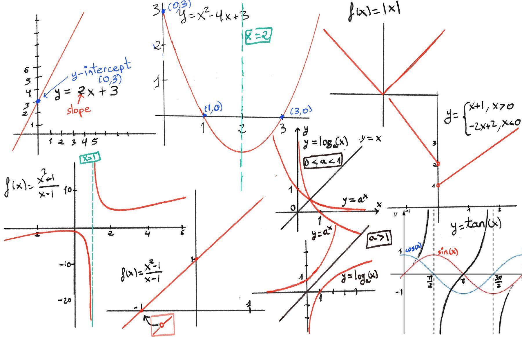
• Absolute value, $f(x) = ∣x∣ = \begin{cases} x, &x \ge 0 \\\\ -x, &x \lt 0 \end{cases}$​. The graph has a sharp vertex (a corner point where the definition changes) at the origin (0, 0). On each side, the function behaves like a straight line with slope +1 for $x \geq 0$ and slope -1 for x < 0. The graph, a V-shaped curve, is symmetric about the y-axis.

• To plot Rational functions $f(x) = \frac{P(x)}{Q(x)}$, determine the domain (exclude points where the denominator is zero), find horizontal, vertical (where Q(x) = 0, say x = a that don’t cancel with P(x) and the function blows up, check one-sided limits $lim _{x \rightarrow a^{\pm}} f(x)$ to see whether it goes to $+\infty$ or $-\infty$), and oblique asymptotes, analyze end behaviour; and possible holes (removable discontinuities where numerator F and denominator Q share a common factor (x - a); cancel it to get the reduced function. The graph follows the reduced function but has a hole at x = a); compute a few points in each interval of the domain and sketch the curve.

  $f(x)=\frac{x^2+1}{x-1}$ has a vertical asymptote x = 1. Behavior near x = 1 (f is not defined at x = 1): $\lim _{x\rightarrow 1^-}f(x)=-\infty$ and $\lim _{x\rightarrow 1^+}f(x)=+\infty$. $g(x)=\frac{x^2-1}{x-1}=\frac{(x-1)(x+1)}{x-1}$ has a hole (removable discontinuity). Cancel to get the reduced function $g_{\mathrm{red}}(x)=x+1$. The graph is the line y = x + 1 with a hole at x = 1 where the function is not defined.

• Exponential $a^x, a \gt 0, a \ne 1$; domain = $\mathbb{R}$ and range = (0, $\infin$), horizontal asymptote: y = 0; Monotonicity: If a > 1: Increasing (exponential growth). If 0 < a < 1: Decreasing (exponential decay); passes through (0, 1);

• Logarithm $log_a(x), a \gt 0, a \ne 1$; domain = (0, $\infin$) and range = $\mathbb{R}$; vertical asymptote: x = 0; Monotonicity: If a > 1: Increasing. If 0 < a < 1: Decreasing; and passes through (1, 0); $log_a(x)$ is the inverse of $a^x$. Their graphs are reflections across the line y = x..

• Trigonometric functions are periodic. sin(x) and cos(x) are smooth, bounded oscillations between -1 and 1 (they have period 2π and range [−1, 1]). sin(x) is an odd function $\sin (-x)=-\sin (x)$ and cos(x) is an even function $\cos (-x)=\cos (x)$. tan(x) has period π, with vertical asymptotes at odd multiples of $\frac{\pi}{2}$. It repeats every $\pi$, shooting off to infinity near its vertical asymptotes.

• Piecewise-defined functions. A piecewise function behaves differently in different regions of the domain, e.g., $f(x) = \begin{cases} x + 1, &x > 0 \\\\ -2x + 2, &x < 0 \end{cases}$. Treat each piece as its own function on its own interval and graph it only on its specified interval. Pay careful attention to open vs closed endpoints. Use a solid or an open dot at a point whether the function is defined or not. Piecewise graphs often show jumps, corners, or different slopes in different regions.

  The graph shows a jump discontinuity at x = 0. The left-hand limit approaches 2, while the right-hand limit approaches 1. Since the function is not defined at x=0, the discontinuity is emphasized by the open circles.

     

Bibliography

1. NPTEL-NOC IITM, Introduction to Galois Theory.
2. Algebra, Second Edition, by Michael Artin.
3. LibreTexts, Calculus. Abstract and Geometric Algebra, Abstract Algebra: Theory and Applications (Judson).
4. Field and Galois Theory, by Patrick Morandi. Springer.
5. Michael Penn, Andrew Misseldine, blackpenredpen, and MathMajor, YouTube’s channels.
6. Contemporary Abstract Algebra, Joseph, A. Gallian.
7. MIT OpenCourseWare, 18.01 Single Variable Calculus, Fall 2007 and 18.02 Multivariable Calculus, Fall 2007, YouTube.
8. Calculus Early Transcendentals: Differential & Multi-Variable Calculus for Social Sciences.