Statistics III. T-tests, Correlations, Linear, and Multilinear Regression

One-Sample and Two-Samples T-tests

Unpaired Two-Samples T-tests are used to compare the means of two independent (unrelated or unpaired) groups.

For example, let’s use rnorm to generate two vectors of normally distributed random numbers (x=rnorm(100), y=rnorm(100), if it is not specified as arguments, mean = 0, sd = 1). t.test(x, y) performs a two-samples t-test comparing the means of two independent samples (x, y, H₀: m_x = m_y or m_x - m_y = 0 ). By default, alternative=“two.sided” H_a: m_x - m_y ≠ 0. p-value = 0.2162 is not inferior or equal to the significance level 0.05, so we can not reject the null hypothesis.

However, x2=rnorm(100, 2) (we generate a vector of normally distributed random numbers with mean = 2 and sd = 1). t.test(x, x2) performs a two-samples t-test comparing the means of x and x2. p-value < 2.2e-16 is inferior to the significance level 0.05, so we can reject the null hypothesis. In other words, we can conclude that the mean values of x and x2 are significantly different.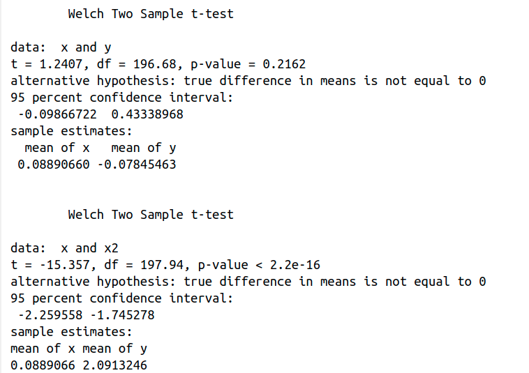

Let’s be a bit more rigorous.

x = rnorm (100)
y = rnorm (100)

First, we must consider that the unpaired two-samples t-test can only be used when the two groups of samples are normally distributed (shapiro_test(x) returns p.value = 0.8622367 > 0.05 and shapiro_test(y) returns p.value = 0.1753192 > 0.05), so the distribution of the data are not significantly different from the normal distribution. Therefore, we can assume normality. Besides, both variances should be equal.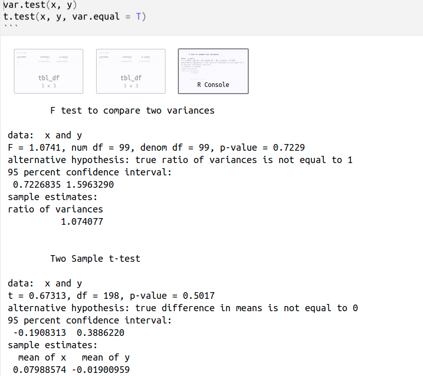

var.test(x, y) performs an F test to compare the variances of two samples. The p-value of the F test = 0.7229 > 0.05, so there is no significant difference between the variances of both samples, we can assume equality of the two variances.

t.test(x, y, var.equal = T) performs a two sample t-test assuming equal variances, p-value = 0.5017 > 0.05, so we can not reject the null hypothesis, H₀: m_x = m_y or m_x - m_y = 0.

x=rnorm(100)
y=rnorm(100, mean=2)
var.test(x, y)
t.test(x, y, var.equal = T)

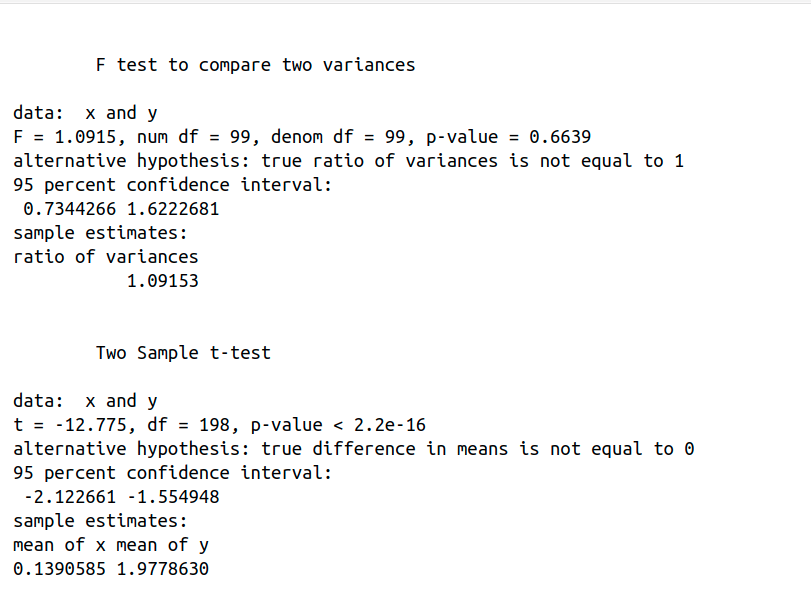
var.test(x, y) performs an F test to compare the variances of two samples. The p-value of the F test = 0.6639 > 0.05, so there is no significant difference between the variances of both samples and we can assume equality of variances . However, t.test(x, y, var.equal = T) performs a two sample t-test, p-value < 2.2e-16, so we can reject the null hypothesis and conclude that the mean values of groups x and y are significantly different.

Let’s take data from the book Probability and Statistics with R: install.packages(“PASWR”) (install.packages installs a given package), library(“PASWR”) (library loads a given package, i.e. attaches it to the search list on your R workspace). Fertilize shows a data frame of plants’ heights in inches obtained from two seeds, one obtained by cross-fertilization and the other by auto fertilization.

   cross   self
1  23.500 17.375
2  12.000 20.375
3  21.000 20.000
4  22.000 20.000
5  19.125 18.375
6  21.500 18.625
7  22.125 18.625
8  20.375 15.250
9  18.250 16.500
10 21.625 18.000
11 23.250 16.250
12 21.000 18.000
13 22.125 12.750
14 23.000 15.500
15 12.000 18.000

> names(Fertilize) # names is a funtion to get the names of the variables of the data frame 
Fertilize [1] "cross" "self"

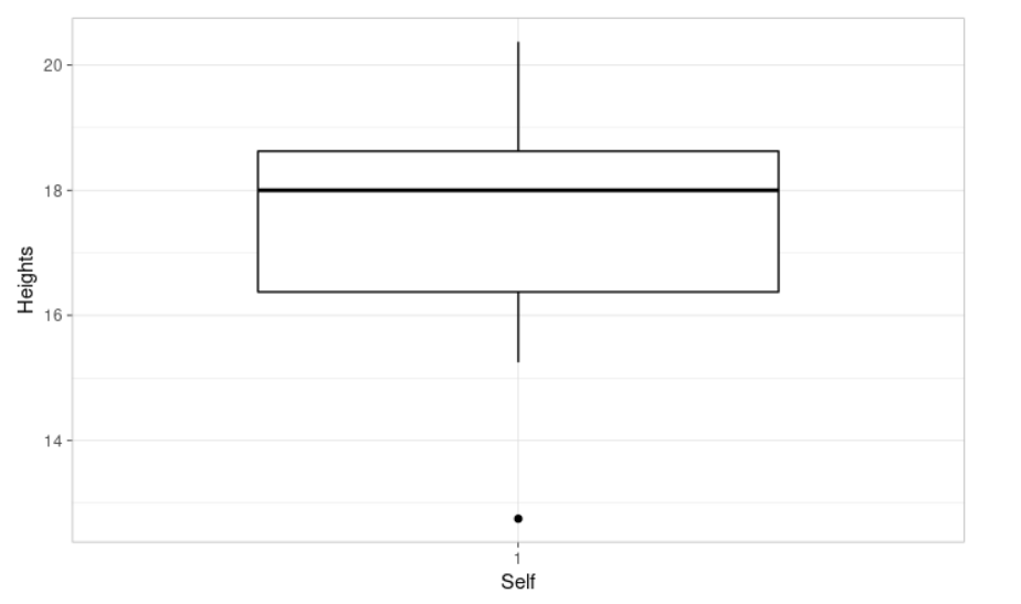
> summary(self) # summary is a function to produce statistical summaries of self: Min (the minimum value), 1st Qu. (the first quartile), Median (the median value), Mean, 3rd Qu. (the third quartile), and Max (the maximum value)
   Min. 1st Qu.  Median    Mean 3rd Qu.    Max. 
  12.75   16.38   18.00   17.57   18.62   20.38

library(ggpubr) 
ggboxplot(self, xlab = "Self", ylab = "Heights", # Let's plot our data 
ggtheme = theme_light()) # We use it to tweak the display

A one-sample t-test is used to compare the mean of one sample to a known value (μ). We can define the null hypothesis as H₀: m = μ. The corresponding alternative hypothesis is H_a: m ≠ μ. It assumes that the data have a normal distribution. Let’s check it.

> shapiro.test(self)

	Shapiro-Wilk normality test

data:  self
W = 0.93958, p-value = 0.3771

We use the Shapiro-Wilk normality test. The null hypothesis is the following, H₀: the data are normally distributed. The corresponding alternative hypothesis is H_a: the data are not normally distributed.

From the output shown below, the p-value = 0.3771 > 0.05 implying that we cannot reject the null hypothesis, the distribution of the data is not significantly different from a normal distribution, and therefore we can assume that the data have a normal distribution.

ggqqplot(self, ylab = "Self", # We use a Q-Q (quantile-quantile) plot (it draws the correlation between a given sample and the theoretical normal distribution). It allows us to visually evaluate the normality assumption. 
ggtheme = theme_minimal())

We want to know if the average plants’ heights in inches obtained by auto fertilization is 17.

> t.test(self, mu=17, conf=.95)

	One Sample t-test

data:  self
t = 1.0854, df = 14, p-value = 0.2961
alternative hypothesis: true mean is not equal to 17
95 percent confidence interval:
 16.43882 18.71118
sample estimates:
mean of x 
   17.575

The value of the t test statistics is 1.0854, its p-value is 0.2961, which is greater than the significance level 0.05. We have no reason to reject the null hypothesis, H₀: m = 17. It also gives us a confidence interval for the mean: [16.43882, 18.71118]. Observe that the hypothesized mean µ = 17 falls into the confidence interval.

Next, we want to know if the mean of the plants heights obtained by cross-fertilization is significantly different from the one obtained by auto fertilization.

> summary(cross) # summary is a function to produce statistical summaries of cross: Min (the minimum value), 1st Qu. (the first quartile), Median (the median value), Mean, 3rd Qu. (the third quartile), and Max (the maximum value)
   Min. 1st Qu.  Median    Mean 3rd Qu.    Max. 
  12.00   19.75   21.50   20.19   22.12   23.50  
> library(ggpubr)
> boxplot(cross, self, ylab = "Height", xlab = "Method") # Let's plot our data

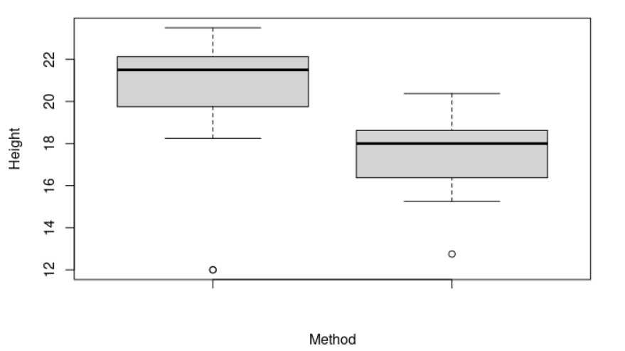
From the plot shown below, we can see that both samples have very different means. Do the two samples have the same variances?

> var.test(cross, self)

	F test to compare two variances

data:  cross and self
F = 3.1079, num df = 14, denom df = 14, p-value = 0.04208
alternative hypothesis: true ratio of variances is not equal to 1
95 percent confidence interval:
 1.043412 9.257135
sample estimates:
ratio of variances 
          3.107894

var.test(cross, self) performs an F test to compare the variances of two samples. The p-value of the F test = 0.04208 < 0.05, so there is a significant difference between the variances of both samples, we can not assume equality of the two variances.

We noted previously that one of the assumptions for the t-test is that the variances of the two samples should be equal. However, a modification of the t-test known as Welch’s test is used to solve this problem. It is actually the default in R, but it can also be specified with the argument var.equal=FALSE.

> t.test(cross, self, conf=.95)

	Welch Two Sample t-test

data:  cross and self
t = 2.4371, df = 22.164, p-value = 0.02328
alternative hypothesis: true difference in means is not equal to 0
95 percent confidence interval:
 0.3909566 4.8423767
sample estimates:
mean of x mean of y 
 20.19167  17.57500

The value of the Welch two sample t-test is 2.4371, its p-value is 0.02328 < 0.05, which is lesser than the significance level 0.05, the null hypothesis is rejected, and therefore we can conclude there is a significant difference between both means.

> shapiro.test(cross) # However, we have not check that the data from the "cross" sample follow a normal distribution

	Shapiro-Wilk normality test

data:  cross
W = 0.753, p-value = 0.0009744 # From the output, p-value = 0.0009744 < 0.05 implying that the distribution of the data is significantly different from the normal distribution. In other words, we can not assume normality.

> wilcox.test(self, cross, exact=FALSE) # If the data are not normally distributed, it’s recommended to use the non-parametric two-samples Wilcoxon test.

	Wilcoxon rank sum test with continuity correction

data:  self and cross
W = 39.5, p-value = 0.002608
alternative hypothesis: true location shift is not equal to 0

The p-value of the test is 0.002608, which is lesser than the significance level alpha = 0.05. We can conclude that the mean of the plants heights obtained by cross-fertilization is significantly different from the mean of the plants obtained by auto fertilization.

Violence in the media

“Virtually since the dawn of television, parents, teachers, legislators, and mental health professionals have wanted to understand the impact of television programs, particularly on children,” Violence in the media: Psychologists study potential harmful effects, American Psychological Association. More specifically, we want to assess the impact of watching violent programs on the viewers.

library("PASWR") # It loads the PASWR package 
attach(Aggression) 

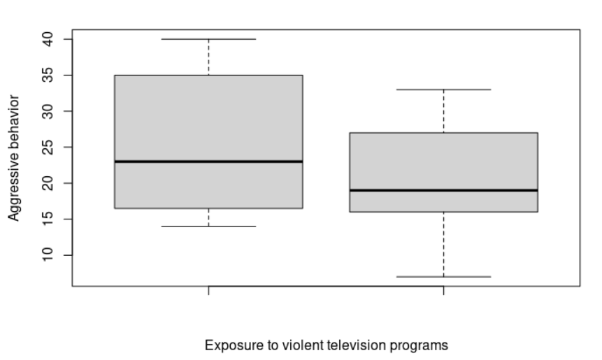
A data frame regarding aggressive behavior in relation to exposure to violent television programs. In each of the resulting 16 pairs, one child is randomly selected to view the most violent shows on TV (violence), while the other watches cartoons, situation comedies, and the like (noviolence).

Aggression # It shows the data frame in a tabular format 

> summary(violence) 

summary is a function to produce statistical summaries of violence: Min (the minimum value), 1st Qu. (the first quartile), Median (the median value), Mean, 3rd Qu. (the third quartile), and Max (the maximum value)

   Min. 1st Qu.  Median    Mean 3rd Qu.    Max. 
  14.00   16.75   23.00   25.12   35.00   40.00 
> summary(noviolence)
   Min. 1st Qu.  Median    Mean 3rd Qu.    Max. 
   7.00   16.00   19.00   20.56   26.50   33.00 
> library(ggpubr)
> boxplot(violence, noviolence, ylab="Aggressive behavior", xlab="Exposure to violent television programs") # Let's plot our data

> shapiro.test(violence)

	Shapiro-Wilk normality test

data:  violence
W = 0.89439, p-value = 0.06538

> shapiro.test(noviolence)

	Shapiro-Wilk normality test

data:  noviolence
W = 0.94717, p-value = 0.4463

From the output shown below, the p-value are 0.06538 and 0.4463, they are both greater than the significant level of 0.05 implying that we cannot reject the null hypothesis, the distribution of the data is not significantly different from a normal distribution in both conditions (violence and noviolence), and therefore we can assume that the data have a normal distribution.

> var.test(violence, noviolence)

	F test to compare two variances

data:  violence and noviolence
F = 1.4376, num df = 15, denom df = 15, p-value = 0.4905
alternative hypothesis: true ratio of variances is not equal to 1
95 percent confidence interval:
 0.5022911 4.1145543
sample estimates:
ratio of variances 
          1.437604

var.test(violence, noviolence) performs an F test to compare the variances of two samples. The p-value of the F test = 0.4905 > 0.05, so there is no significant difference between the variances of both samples, we can assume equality of the two variances.

> t.test(violence, noviolence)

	Welch Two Sample t-test

data:  violence and noviolence
t = 1.5367, df = 29.063, p-value = 0.1352
alternative hypothesis: true difference in means is not equal to 0
95 percent confidence interval:
 -1.509351 10.634351
sample estimates:
mean of x mean of y 
  25.1250   20.5625 

> t.test(violence, noviolence, var.equal = T)

	Two Sample t-test

data:  violence and noviolence
t = 1.5367, df = 30, p-value = 0.1349
alternative hypothesis: true difference in means is not equal to 0
95 percent confidence interval:
 -1.501146 10.626146
sample estimates:
mean of x mean of y 
  25.1250   20.5625 

t.test(violence, noviolence, var.equal = T) performs a two sample t-test assuming equal variances, p-value = 0.1349 > 0.05, so we can not reject the null hypothesis. We can conclude that there is no statistically significant difference regarding to violence in relation to exposure to violent television programs. I want you to observe that the Welch statistics produce similar results.

Correlation tests in R

Variables within a dataset can be related for lots of reasons. One variable could cause or depend on the values of another variable, or they could both be effects of a third variable. The statistical relationship between two variables is referred to as their correlation and a correlation test is used to evaluate the association between two or more variables.

A correlation could be positive, meaning both variables change or move either up or down in the same direction together (an example would be height and weight, taller people tend to be heavier), or negative, meaning that when one variable’s values increase, the other variable’s values decrease and vice versa (an example would be exercise and weight, the more you exercise, the less you will weigh). Correlation can also be zero, meaning that the variables are unrelated or independent of each other. For example, there is no relationship between the amount of Coke drunk by the average person and his or her level of income or earnings.

A correlation coefficient measures the strength of the relationship between two variables. There are three types of correlation coefficients: Pearson, Spearman, and Kendall. The most widely used is the Pearson correlation. It measures a linear dependence between two variables.

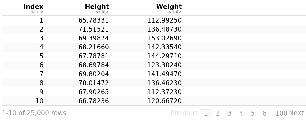
Let’s use a dataset from the Statistics Online Computational Resource (SOCR). It contains the height (inches) and weights (pounds) of 25,000 different humans of 18 years of age. The file SOCR-HeightWeight.csv reads as follows:

Index,Height,Weight # Initially, the first line was Index, Height(Inches), Weight(Pounds)
1,65.78331,112.9925
2,71.51521,136.4873
3,69.39874,153.0269
4,68.2166,142.3354
5,67.78781,144.2971
6,68.69784,123.3024
7,69.80204,141.4947
8,70.01472,136.4623
9,67.90265,112.3723 […]

weightHeight <- read.table("/path/SOCR-HeightWeight.csv", header = T, sep = “,”) # read.table loads our file into R, we use sep = “,” to specify the separator character. weightHeight

library("ggpubr")
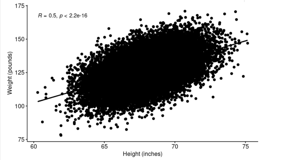
ggscatter(weightHeight, x = "Height", y = "Weight", # Let's draw our data, x and y are the variables for plotting
          add = "reg.line", conf.int = TRUE, # add = "reg.line" adds the regression line, and conf.int = TRUE adds the confidence interval.
          cor.coef = TRUE, cor.method = "pearson", # cor.coef = TRUE adds the correlation coefficient with the p-value, cor.method = "pearson" is the method for computing the correlation coefficient. 
          xlab = "Height (inches)", ylab = "Weight (pounds)")

> shapiro.test(weightHeight$Height[0:5000]) # We can see from the plot above, the relationship is linear. 

Do our data (Weight, Height) follow a normal distribution? Shapiro test cannot deal with more than 5.000 data points. We are going to do the shapiro test using only the first 5.000 samples.

	Shapiro-Wilk normality test

data:  weightHeight$Height[0:5000]
W = 0.99955, p-value = 0.2987
> shapiro.test(weightHeight$Weight[0:5000])

	Shapiro-Wilk normality test

data:  weightHeight$Weight[0:5000]
W = 0.99979, p-value = 0.9355

From the output above, the two p-values (0.2987, 0.9355) are greater than the significance level 0.05. Thus, we cannot reject the null hypothesis, the distributions of the data from each of the two variables are not significantly different from the normal distribution. In other words, we can assume normality.

We can use Q-Q plots to visualize the correlation between each of the two variables and the normal distribution: library(“ggpubr”), ggqqplot(weightHeight$Height, ylab = “Height”), ggqqplot(weightHeight$Weight, ylab = “Weight”).

> cor.test(weightHeight$Height, weightHeight$Weight)

	Pearson's product-moment correlation

data:  weightHeight$Height and weightHeight$Weight
t = 91.981, df = 24998, p-value < 2.2e-16
alternative hypothesis: true correlation is not equal to 0
95 percent confidence interval:
 0.4935390 0.5120626
sample estimates:
      cor 
0.5028585

cor.test performs a correlation test between two variables. It returns both the correlation coefficient and the significance level(or p-value) of the correlation. The t-test statistic value is 91.981, its p-value is < 2.2e-16 so we can conclude that Height and Weight are positively significant correlated (r = 0.5028585, p-value < 2.2e-16).

Linear Regression in R

Linear regression is a model to estimate or analyze the relationship between a dependent or response variable (often called or denoted as y) and one or more independent or explanatory variables (often called x). In other words, linear regression predicts a value for Y, ‘given’ a value of X.

It assumes that there exists a linear relationship between the response variable and the explanatory variables. Graphically, a linear relationship is a straight line when plotted as a graph. Its general equation is y = b₀ + b₁*x + e where y is the response variable, x is the predictor, independent, or explanatory variable, b₀ is the intercept of the regression line (the predicted value when x=0) with the y-axis, b₁ is the slope of the regression line, and e is the error term or the residual error (the part of the response variable that the regression model is unable to explain).

Let’s use our dataset from the Statistics Online Computational Resource (SOCR). It contains the height (inches) and weights (pounds) of 25,000 different humans of 18 years of age.

weightHeight <- read.table("/path/SOCR-HeightWeight.csv", header = T, sep = ",") 
# read.table loads our file into R, we use sep = "," to specify the separator character. 
weightHeight

library("ggpubr")
ggscatter(weightHeight, x = "Height", y = "Weight", # Let's draw our data, x and y are the variables for plotting
          add = "reg.line", conf.int = TRUE, # add = "reg.line" adds the regression line, and conf.int = TRUE adds the confidence interval.
          cor.coef = TRUE, cor.method = "pearson", # cor.coef = TRUE adds the correlation coefficient with the p-value, cor.method = "pearson" is the method for computing the correlation coefficient. 
          xlab = "Height (inches)", ylab = "Weight (pounds)")

The graph above strongly suggests a linearly relationship between Height and Weight.

> cor.test(weightHeight$Height, weightHeight$Weight)

	Pearson's product-moment correlation

data:  weightHeight$Height and weightHeight$Weight
t = 91.981, df = 24998, p-value < 2.2e-16
alternative hypothesis: true correlation is not equal to 0
95 percent confidence interval:
 0.4935390 0.5120626
sample estimates:
      cor 
0.5028585

The correlation coefficient measures the strength of the relationship between two variables x and y. A correlation coefficient of r=.50 indicates a stronger degree of a linear relationship than one of r=.40. Its value ranges between -1 (perfect negative correlation) and +1 (perfect positive correlation).

If the coefficient is, say, .80 or .95, we know that the corresponding variables closely vary together in the same direction. Otherwise, if it were -.80 or -.95, x and y would vary together in opposite directions. A value closer to 0 suggests a weak relationship between the variables, they vary separately. A low correlation (-0.2 < x < 0.2) suggests that much of the variation of the response variable (y) is not explained by the predictor (x) and we need to look for better predictor variables.

Observe that the correlation coefficient (0.5028585) is good enough but far from perfect, so we can continue with our study.

> model <- lm(Weight ~ Height, data = weightHeight)
> summary(model)

Call:
lm(formula = Weight ~ Height, data = weightHeight)

Residuals:
    Min      1Q  Median      3Q     Max 
-40.302  -6.711  -0.052   6.814  39.093 

Coefficients:
             Estimate Std. Error t value Pr(>|t|)    
(Intercept) -82.57574    2.28022  -36.21   <2e-16 ***
Height        3.08348    0.03352   91.98   <2e-16 ***
---
Signif. codes:  0 ‘***’ 0.001 ‘**’ 0.01 ‘*’ 0.05 ‘.’ 0.1 ‘ ’ 1

Residual standard error: 10.08 on 24998 degrees of freedom
Multiple R-squared:  0.2529,	Adjusted R-squared:  0.2528 
F-statistic:  8461 on 1 and 24998 DF,  p-value: < 2.2e-16

A linear regression can be calculated in R with the command lm. The command format is as follows: lm([target variable] ~ [predictor variables], data = [data source]). We can see the values of the intercept and the slope. Therefore, the regression line equation can be written as follows: Weight = -82.57574 + 3.08348*Height.

One measure to test how good is the model is the coefficient of determination or R². For models that fit the data very well, R² is near to 1. In other words, you have a very tight correlation and can predict y quite precisely if you know x. On the other side, models that poorly fit the data have R² near 0. In our example, the model only explains 25.28% of the data variability. The F-statistic (8461) gives the overall significance of the model, it produces a model p-value < 2.2e-16 which is highly significant.

The p-Value of individual predictor variables (extreme right column under ‘Coefficients’) are very important. When there is a p-value, there is a null and alternative hypothesis associated with it. The null hypothesis H₀ is that the coefficients associated with the variables are equal to zero (i.e., no relationship between x and y). The alternate hypothesis H_a is that the coefficients are not equal to zero (i.e., there is some relationship between x and y). In our example, both the p-values for the Intercept and Height (the predictor variable) are significant, so we can reject the null hypothesis, there is a significant relationship between the predictor (Height) and the outcome variable (Weight).

The residual data of the linear regression model is the difference between the observed data of the dependent variable y and the fitted values ŷ (the predicted response values given the values for our explanatory variables). We can plot them: plot(model$residuals) and they should look random.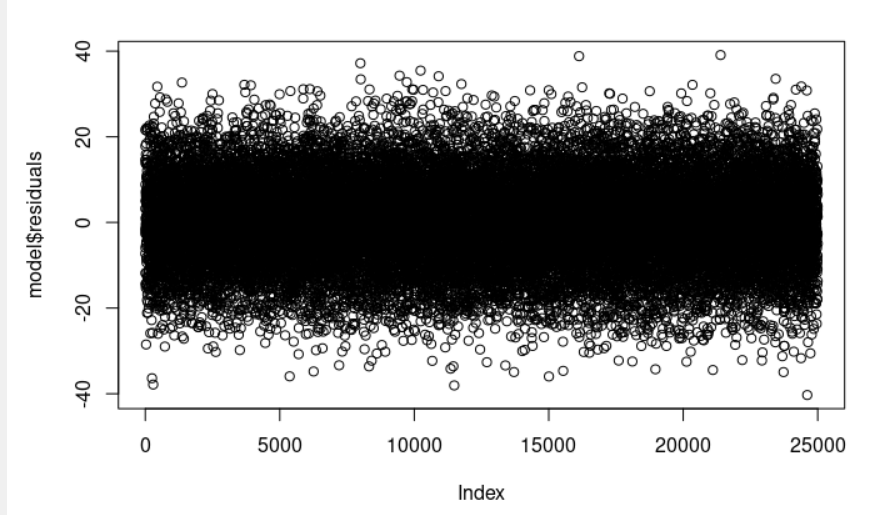

Observe that the section residuals (model <- lm(Weight ~ Height, data = weightHeight), summary(model)) provides a quick view of the distribution of the residuals. The median (-0.052) is close to zero, and the minimum and maximum values are roughly equal in absolute value (-40.302, 39.093).

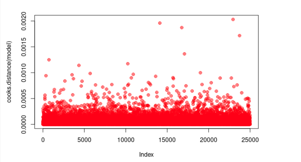
plot(cooks.distance(model), pch = 10, col = "red") # Cook's distance is used in Regression Analysis to find influential points and outliers. It’s a way to identify points that negatively affect the regression model. We are going to plot them.
cook <- cooks.distance(model)
significantValues <- cook > 1 # As a general rule, cases with a Cook's distance value greater than one should be investigated further. 
significantValues # We get none of those points.

Multiple linear regression

Multiple linear regression is an extension of simple linear regression that uses several explanatory variables (predictor or independent variables) to predict the outcome of a response variable (outcome or dependent variable).

Its general equation is *y = b₀ + b₁x1 + b₂x2 + b₃x3 + … + + b_nxn +e where y is the response or dependent variable, xi are the predictor, independent, or explanatory variables, b₀ is the intercept of the regression line with the y-axis (the predicted value when all xi=0), b₁ is the regression coefficient of the first independent variable x1,… b_n is the regression coefficient of the last independent variable xn and e is the error term or the residual error (the part of the response variable that the regression model is unable to explain).

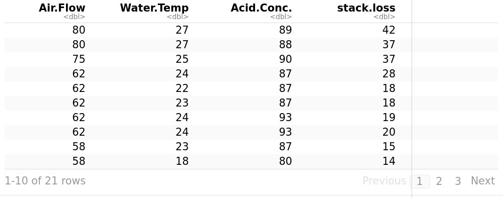
Let’s use stackloss. It is described as operational data of a plant for the oxidation of ammonia to nitric acid. stack.loss is the dependent variable, it is the percentage of the ingoing ammonia to the plant that escapes from the absorption column unabsorbed; that is, an (inverse) measure of the over-all efficiency of the plant. Air Flow is the flow of cooling air. It represents the rate of operation of the plant. Water Temp is the temperature of cooling water circulated through coils in the absorption tower.

> stackloss

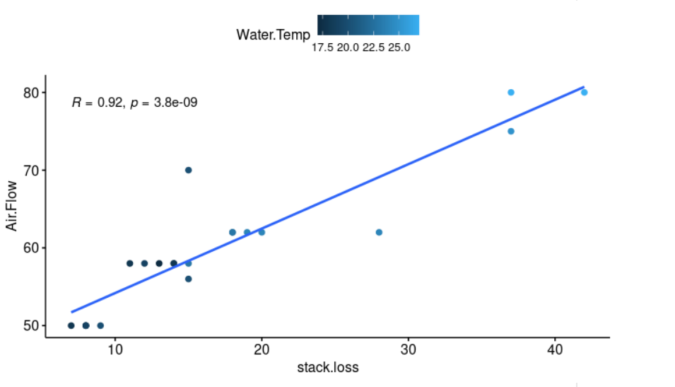
library("ggpubr")
ggscatter(stackloss, x = "stack.loss", y = "Air.Flow", color = "Water.Temp" # Let's plot our data, we can also add color to our datapoints based on the second factor (color="Water.Temp")
          add = "reg.line", conf.int = TRUE, # add = "reg.line" adds the regression line, and conf.int = TRUE adds the confidence interval.
          cor.coef = TRUE, cor.method = "pearson", # cor.coef = TRUE adds the correlation coefficient with the p-value, cor.method = "pearson" is the method for computing the correlation coefficient. 
          xlab = "stack.loss", ylab = "Air.Flow")

A linear regression can be calculated in R with the command lm. The command format is as follows: lm([target variable] ~ [predictor variables], data = [data source]).

> model <- lm(stack.loss ~ Air.Flow + Water.Temp, data = stackloss)
> summary(model)

Call:
lm(formula = stack.loss ~ Air.Flow + Water.Temp, data = stackloss)

Residuals:
    Min      1Q  Median      3Q     Max 
-7.5290 -1.7505  0.1894  2.1156  5.6588 

Coefficients:
            Estimate Std. Error t value Pr(>|t|)    
(Intercept) -50.3588     5.1383  -9.801 1.22e-08 ***
Air.Flow      0.6712     0.1267   5.298 4.90e-05 ***
Water.Temp    1.2954     0.3675   3.525  0.00242 ** 
---
Signif. codes:  0 ‘***’ 0.001 ‘**’ 0.01 ‘*’ 0.05 ‘.’ 0.1 ‘ ’ 1

Residual standard error: 3.239 on 18 degrees of freedom
Multiple R-squared:  0.9088,	Adjusted R-squared:  0.8986 
F-statistic: 89.64 on 2 and 18 DF,  p-value: 4.382e-10

The regression line equation can be written as follows: stack.loss = -50.3588 + 0.6712*Air.Flow + 1.2954*Water.Temp.

One measure to test how good is the model is the coefficient of determination or R². For models that fit the data very well, R² is close to 1. On the other side, models that poorly fit the data have R² near to 0. In our example, the model explains 89.86% of the data variability. In other words, it explains quite a lot of the variance in the dependent variable. The F-statistic (89.64) gives the overall significance of the model, it produces a model p-value: 4.382e-10 which is highly significant.

The p-Value of individual predictor variables (extreme right column under ‘Coefficients’) are very important. When there is a p-value, there is a null and alternative hypothesis associated with it. The null hypothesis H₀ is that the coefficients associated with the variables are equal to zero (i.e., no relationship between xi and y). The alternate hypothesis H_a is that the coefficients are not equal to zero (i.e., there is some relationship between xi and y). In our example, both the p-values for the Intercept, Air.Flow, and Water.Temp (the predictor variables) are significant, so we can reject the null hypothesis, there is a significant relationship between the predictors (Air.Flow, Water.Temp) and the outcome variable (stack.loss).

The residual data of the linear regression model is the difference between the observed data of the dependent variable y and the fitted values ŷ. We can plot them: plot(model$residuals) and they should look random.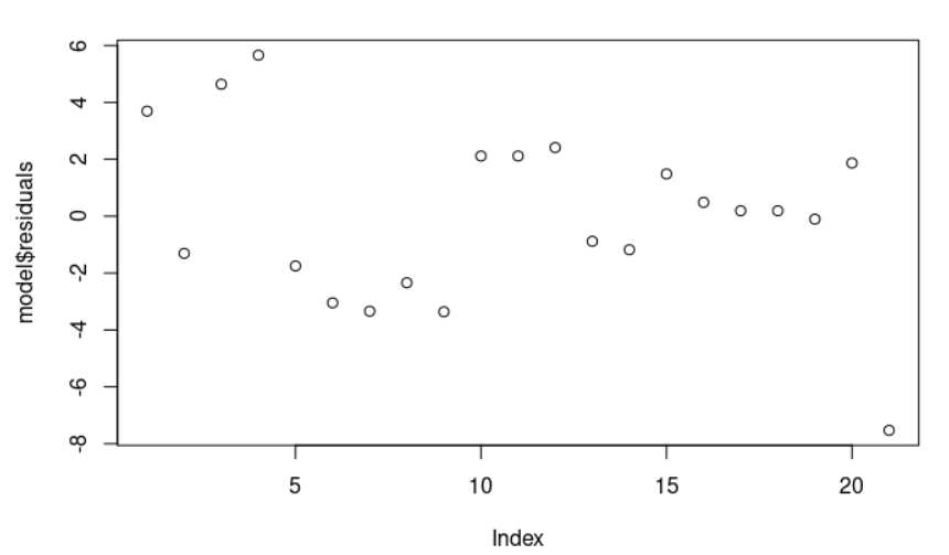

Observe that the section residuals (model <- lm(stack.loss ~ Air.Flow + Water.Temp, data = stackloss), summary(model)) provides a quick view of the distribution of the residuals. The median (0.1894) is close to zero, and the minimum and maximum values are somehow close in absolute magnitude (-7.5290, 5.6588 ).

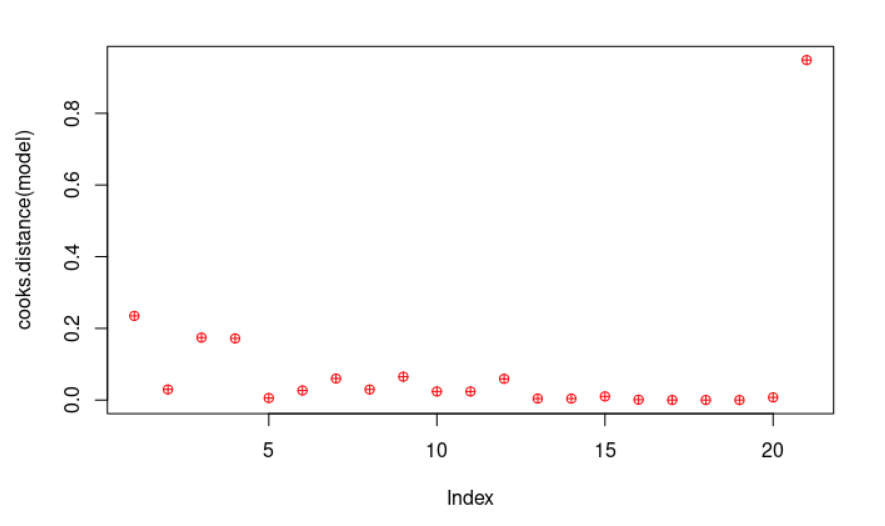
plot(cooks.distance(model), pch = 10, col = "red") # Cook's distance is used in Regression Analysis to find influential points and outliers. It’s a way to identify points that negatively affect the regression model. We are going to plot them.
cook <- cooks.distance(model)
significantValues <- cook > 1 # As a general rule, cases with a Cook's distance value greater than one should be investigated further. 
significantValues # We get none of those points.
1     2     3     4     5     6     7     8     9    10    11    12    13    14    15 
FALSE FALSE FALSE FALSE FALSE FALSE FALSE FALSE FALSE FALSE FALSE FALSE FALSE FALSE FALSE 
   16    17    18    19    20    21 
FALSE FALSE FALSE FALSE FALSE FALSE

Let’s see another example of multiple linear regression using Edgar Anderson’s Iris Data.

> data(iris) 

The iris data set gives the measurements in centimeters of the variables sepal length and width and petal length and width, respectively, for 50 flowers from each of 3 species of iris.

> summary(iris)
  Sepal.Length    Sepal.Width     Petal.Length    Petal.Width          Species  
 Min.   :4.300   Min.   :2.000   Min.   :1.000   Min.   :0.100   setosa    :50  
 1st Qu.:5.100   1st Qu.:2.800   1st Qu.:1.600   1st Qu.:0.300   versicolor:50  
 Median :5.800   Median :3.000   Median :4.350   Median :1.300   virginica :50  
 Mean   :5.843   Mean   :3.057   Mean   :3.758   Mean   :1.199                  
 3rd Qu.:6.400   3rd Qu.:3.300   3rd Qu.:5.100   3rd Qu.:1.800                  
 Max.   :7.900   Max.   :4.400   Max.   :6.900   Max.   :2.500                  
> model <- lm(Sepal.Length ~ Sepal.Width + Petal.Length + Petal.Width, data = iris)
> summary(model)

Call:
lm(formula = Sepal.Length ~ Sepal.Width + Petal.Length + Petal.Width, 
    data = iris)

Residuals:
     Min       1Q   Median       3Q      Max 
-0.82816 -0.21989  0.01875  0.19709  0.84570 

Coefficients:
             Estimate Std. Error t value Pr(>|t|)    
(Intercept)   1.85600    0.25078   7.401 9.85e-12 ***
Sepal.Width   0.65084    0.06665   9.765  < 2e-16 ***
Petal.Length  0.70913    0.05672  12.502  < 2e-16 ***
Petal.Width  -0.55648    0.12755  -4.363 2.41e-05 ***
---
Signif. codes:  0 ‘***’ 0.001 ‘**’ 0.01 ‘*’ 0.05 ‘.’ 0.1 ‘ ’ 1

Residual standard error: 0.3145 on 146 degrees of freedom
Multiple R-squared:  0.8586,	Adjusted R-squared:  0.8557 
F-statistic: 295.5 on 3 and 146 DF,  p-value: < 2.2e-16

> plot(model$residuals)

The regression line equation can be written as follows: Sepal.Length = 1.85600 + 0.65084*Sepal.Width + 0.70913*Petal.Length + -0.55648*Petal.Width. In this example, the model explains 85.57% of the data variability (it explains quite a lot of the variance in the dependent variable, Sepal.Length). The F-statistic (295.5) gives the overall significance of the model, it produces a model p-value: < 2.2e-16 which is highly significant.

Both the p-values for the Intercept and the individual predictor variables (Sepal.Width, Petal.Length, and Petal.Width) are significant, so we can reject the null hypothesis, there is a significant relationship between the predictors (Sepal.Width, Petal.Length, and Petal.Width) and the outcome variable (Sepal.Length).

The residual data of the linear regression model is the difference between the observed data of the dependent variable y and the fitted values ŷ. We can plot them: plot(model$residuals) and they look random.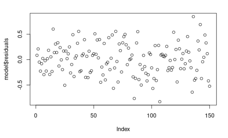

Let’s have a third and last example of multiple linear regression using the trees dataset. It provides measurements of the diameter (it is labelled Girth), height and volume of timber in 31 felled black cherry trees.

> summary(trees)
     Girth           Height       Volume     
 Min.   : 8.30   Min.   :63   Min.   :10.20  
 1st Qu.:11.05   1st Qu.:72   1st Qu.:19.40  
 Median :12.90   Median :76   Median :24.20  
 Mean   :13.25   Mean   :76   Mean   :30.17  
 3rd Qu.:15.25   3rd Qu.:80   3rd Qu.:37.30  
 Max.   :20.60   Max.   :87   Max.   :77.00  
> model <- lm(Volume ~ Girth + Height, data = trees)
> summary(model)

Call:
lm(formula = Volume ~ Girth + Height, data = trees)P

Residuals:
    Min      1Q  Median      3Q     Max 
-6.4065 -2.6493 -0.2876  2.2003  8.4847 

Coefficients:
            Estimate Std. Error t value Pr(>|t|)    
(Intercept) -57.9877     8.6382  -6.713 2.75e-07 ***
Girth         4.7082     0.2643  17.816  < 2e-16 ***
Height        0.3393     0.1302   2.607   0.0145 *  
---
Signif. codes:  0 ‘***’ 0.001 ‘**’ 0.01 ‘*’ 0.05 ‘.’ 0.1 ‘ ’ 1

Residual standard error: 3.882 on 28 degrees of freedom
Multiple R-squared:  0.948,	Adjusted R-squared:  0.9442 
F-statistic:   255 on 2 and 28 DF,  p-value: < 2.2e-16

The regression line equation can be written as follows: Volume = -57.9877 + 4.7082*Girth + 0.3393*Height. In this example, the model explains 94.42% of the data variability. It explains most of the variance in the dependent variable, Volume. The F-statistic (255) gives the overall significance of the model, it produces a model p-value: < 2.2e-16 which is highly significant.

Both the p-values for the Intercept and the individual predictor variables (Girth and Height) are significant, so we can reject the null hypothesis, there is a significant relationship between the predictors (Girth and Height) and the outcome variable (Volume).