
|
 |
 |
|
 |
|
|
|
|
|
|
Everyone knows that smoking is a bad idea. The question that we will try to address in this article is the following: Do smoking habits differ between women and men? We are going to use some data from the . Chi-squared Test of Independence
It defines everyday smokers as current smokers who smoke every day; some-day smokers are current smokers who smoke on some days. Former smokers have smoked at least 100 cigarettes in their lifetime but currently do not smoke at all.
>>> sexSmoke<-rbind(c(13771, 4987, 30803), c(11722, 3674, 24184))
# The rbind() function is used to bind or combine these two vectors by rows.

>>> dimnames(sexSmoke)<-list(c("Male", "Female"), c("Every-day smoker", "Some-day smoker", "Former smoker"))
# The dimnames() command sets the row and column names of a matrix

>>> sexSmoke
           Every-day smoker Some-day smoker Former smoker
Male              13771            4987         30803
Female            11722            3674         24184
> chisq.test(sexSmoke)

	Pearson's Chi-squared test

data:  sexSmoke
X-squared = 43.479, df = 2, p-value = 3.62e-10
The chi-square test of independence is used to determine whether there is a statistically significant difference between the expected and the observed frequencies in one or more categories of a contingency table.
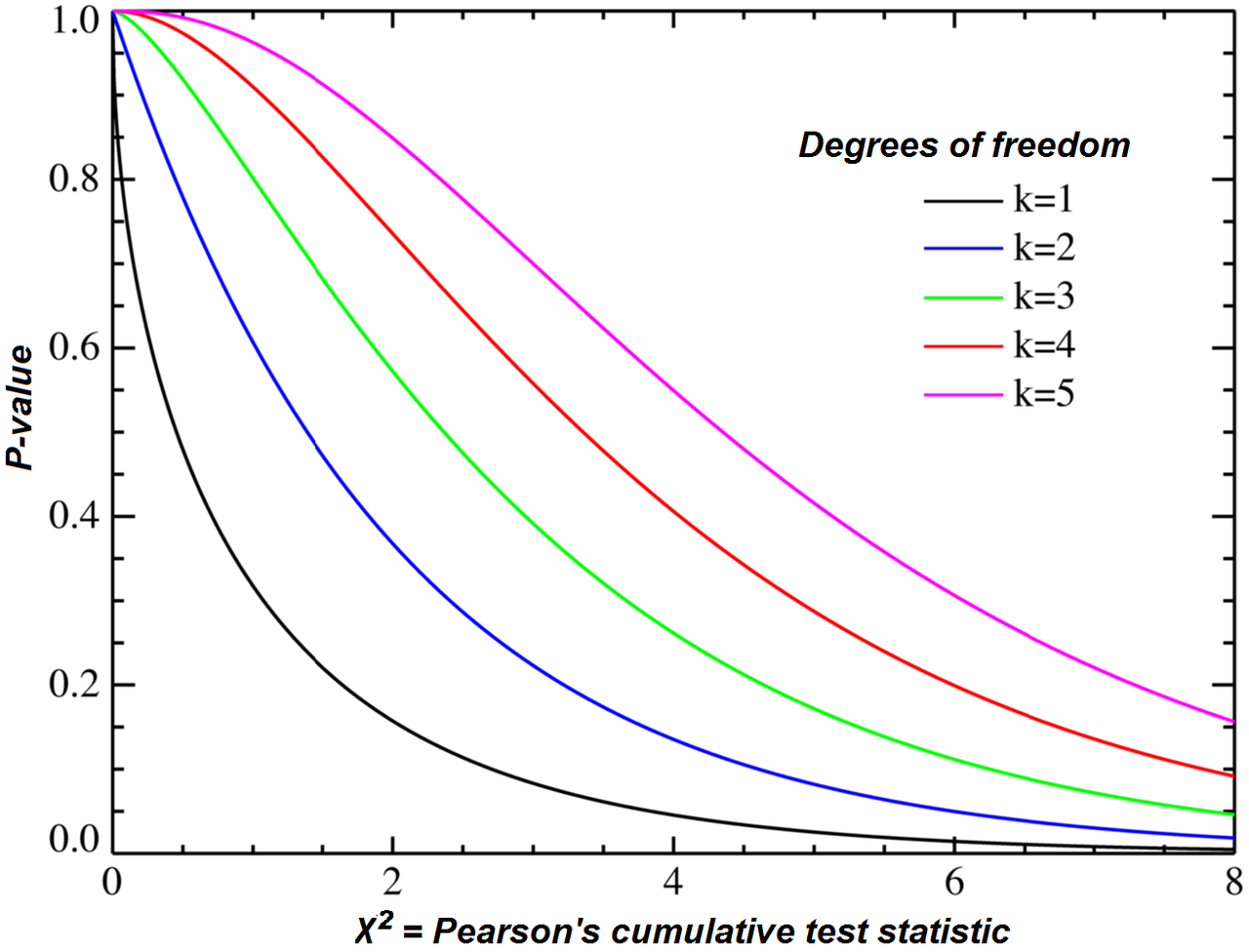
Null hypothesis (H0): the row and the column variables of the contingency table are independent. The test statistic computed from the observations follows a χ2 frequency distribution. The null hypothesis of the independence assumption is to be rejected if the p-value of the Chi-squared test statistic is less than a given significance level α (=0.05).
Alternative hypothesis (H1): the row and the column variables of the contingency table are dependent.
In our example, the p-value of the Chi-squared test statistic = 3.62e-10, the row and the column variables are statistically significantly associated. In other words, smoking habits differ between women and men.
Most people will stop here—but the more adventurous try to understand better the Chi-squared test.
sexSmoke
           Every-day smoker Some-day smoker Former smoker
Male              13771            4987         30803      49561
Female            11722            3674         24184      39580
                  25493            8661         54987      89141
By the assumption of independence under the null hypothesis we should “expect” the number of male every-day smoker to be = 25493 * 49561⁄89141 = 14173.7087648.
>>> chisq<-chisq.test(sexSmoke)
>>> round(chisq$expected, 2) # We can extract the expected counts from the result of the test
       Every-day smoker Some-day smoker Former smoker
Male           14173.71         4815.38      30571.91
Female         11319.29         3845.62      24415.09
What is the difference between the expected and observed results? The difference between the expected and observed count in the “male every day smoker” cell is (observed-expected)2⁄expected = (13771-14173.71)2⁄14173.71 = 11.4419826637.
>>> (chisq$observed-chisq$expected)^2/(chisq$expected)
# We can extract the expected and observed counts from the result of the test and calculate the difference
       Every-day smoker Some-day smoker Former smoker
Male           11.44191        6.116505      1.746773
Female         14.32725        7.658922      2.187262
The sum of these quantities on all cells is the test statistic; in this case, χ2 = ∑(observed-expected)2⁄expected = 43.47863.
>>> m= (chisq$observed-chisq$expected)^2/(chisq$expected)
>>> sum(m)
[1] 43.47863
Under the null hypothesis, this sum has approximately a chi-squared distribution with n = (number of rows-1) (number of columns-1) = (2 - 1) (3 - 1) = 2 degrees of freedom.
The test statistic is improbably large according to that chi-squared distribution, so we should reject the null hypothesis of independence.
The one-way analysis of variance (ANOVA) is used to determine whether there are any statistically significant differences between the means of three or more independent groups. The data is organized into several groups based on one single grouping variable (the factor or independent variable), so there is one categorical independent variable and one quantitative dependent variable.
Imagine that you want to test the effect of three different fertilizer mixtures on crop yield or the effect of three drugs on pain. You can use a one-way ANOVA to find out if there is a difference in crop yields or a difference in pain between the three groups. The independent variable is the type of fertilizer or drug. A pharmaceutical company conducts an experiment to test the effect of its new drug. The company selects some subjects and each subject is randomly assigned to one of three treatment groups where different doses are applied. The drug is the independent variable.
ANOVA test hypotheses:
H0, null hypothesis: μ0 = μ1 = μ2 = … =μk, where μ = group mean and k = number of groups. In other words, the means of the different groups are identical. Ha, alternative hypothesis: At least, the mean of one group is different.
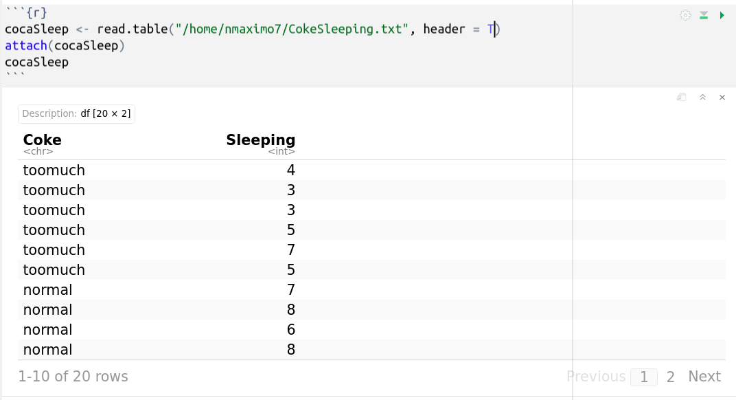
Let’s evaluate the relationship between self-reported sleeping hours and Coke consumption (too much, normal, nothing at all). The data is organized into several groups based on one single grouping variable “Coke consumption” and one quantitative dependent variable “sleeping hours.”
Coke Sleeping
toomuch 4
toomuch 3
toomuch 3
toomuch 5
toomuch 7
toomuch 5
normal 7
normal 8
normal 6
normal 8
normal 7
normal 7
normal 8
normal 8
nothing 7
nothing 8
nothing 7
nothing 8
nothing 8
nothing 9
            Df Sum Sq Mean Sq F value   Pr(>F)
Coke         2  40.34  20.171   18.83 4.88e-05 ***
Residuals   17  18.21   1.071
---
Signif. codes:  0 ‘***’ 0.001 ‘**’ 0.01 ‘*’ 0.05 ‘.’ 0.1 ‘ ’ 1
The output includes the F-value column. This is the test statistic from the F test. The idea behind an ANOVA test relies on estimating the common population variance in two different ways: 1) through the common variance, the mean of the sample variances, which is called the variance within samples or residual variance and denoted S2within, and 2) through the variance of the sample means, which is called the variance between samples means and denoted S2between.
The F-statistic is the ratio of the variance between samples means to the variance within sample means: S2between/S2within. When the means are not significantly different, the variance of the sample means will be small, relative to the mean of the sample variances. When at least one mean is significantly different from the others, the variance of the sample means will be larger, relative to the mean of the sample variances. The larger the F value, the more likely it is that the variation caused by the independent variable is real and not due to chance.
As the p-value is less than the significance level 0.05, there are significant differences between the groups (it is highlighted with an asterisk “*" in the model summary). In other words, the Coke consumption has a real impact on sleeping.
>>> summary(cocaSleep)
Coke              Sleeping
 Length:20          Min.   :3.00
 Class :character   1st Qu.:5.75
 Mode  :character   Median :7.00
                    Mean   :6.65
                    3rd Qu.:8.00
                    Max.   :9.00
>>> tapply(Sleeping, Coke, mean) # computes the mean for each factor variable (Coke) in a vector (Sleeping)
  normal  nothing  toomuch
7.375000 7.833333 4.500000
>>> tapply(Sleeping, Coke, sd)
   normal   nothing   toomuch
0.7440238 0.7527727 1.5165751
Coke Sleeping Meantoomuch
toomuch 4 4.5
toomuch 3 4.5
toomuch 3 4.5
toomuch 5 4.5
toomuch 7 4.5
toomuch 5 4.5
SSwithin = “Sum of squares within groups” = (4-4.5)2 +(3-4.5)2 +(3-4.5)2 +(5-4.5)2 +(7-4.5)2 +(5-4.5)2 + (7-7.375)2 + (8-7.375)2 + (6-7.375)2 +(8-7.375)2 + (7-7.3753)2 +(7-7.375)2 +(8-7.375)2 +(8-7.375)2 + (7-7.83)2 +(8-7.83)2 + (7-7.83)2 + (8-7.83)2 + (8-7.83)2 + (9-7.83)2 = 18.21. MSwithin = SSwithin⁄dfwithin = 18.21⁄17 = 1.07. Finally, F = MSbetween⁄MSwithin = 20.171⁄1.07 = 18.83.
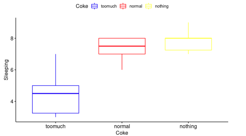
library("ggpubr")
ggboxplot(cocaSleep, x = "Coke", y = "Sleeping",
          color = "Coke", palette = c("blue", "red", "yellow"),
          ylab = "Sleeping", xlab = "Coke")
TukeyHSD(anova)
  Tukey multiple comparisons of means
    95% family-wise confidence level

Fit: aov(formula = Sleeping ~ Coke)

$Coke
                      diff        lwr       upr     p adj
nothing-normal   0.4583333 -0.9755105  1.892177 0.6960429
toomuch-normal  -2.8750000 -4.3088438 -1.441156 0.0002279
toomuch-nothing -3.3333333 -4.8661769 -1.800490 0.0000940
It can be seen from the output’s results (diff is the difference between means of the two groups; lwr and upr are the lower and the upper-end point of the confidence interval; and p adj, p-value after adjustment for the multiple comparisons) that there is significant difference between drinking too much Coke and normal, and drinking too much and nothing.
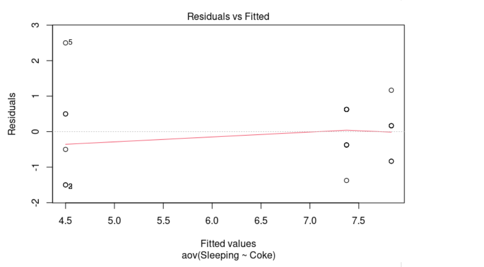
As we can see in the plot above, it looks quite random, there is no evident relationships between residuals and fitted values (the mean of each group). Therefore, we can assume the homogeneity of variances in the different groups. The Levene’s test is also available to check the homogeneity of variances.
library(car)
leveneTest(Sleeping~Coke)

Levene's Test for Homogeneity of Variance (center = median)
      Df F value Pr(>F)
group  2  2.2956 0.1311
      17
“Levene’s test is an inferential statistic used to assess the equality of variances for two or more groups. If the resulting p-value of Levene’s test is less than some significance level (typically 0.05), the obtained differences in sample variances are unlikely to have occurred based on random sampling from a population with equal variances,” Wiki, Levene’s test.
From our result, the p-value 0.1311 > 0.05 so there is no evidence to suggest that the variance across groups is statistically significantly different. In other words, we can assume the homogeneity of variances in the different groups.
A two-way ANOVA is used to estimate how the mean of a quantitative variable changes according to the levels of two categorical variables. It not only aims at assessing the main effect of each independent variable but also if there is any interaction between them.
Hypotheses: H0, null hypothesis: The means of the dependent variable for each group in the first independent variable are equal Ha, alternative hypothesis: The means of the dependent variable for each group in the first independent variable are not equal Similar hypotheses are considered for the other independent variable and the interaction effect.
Let’s determine if there is a statistically significant difference in “Sleeping hours” based on Coke consumption (too much, normal, nothing at all) and gender. The data is organized based on two grouping independent variables “Coke consumption” and “Gender”, and one quantitative dependent variable “Sleeping hours.” CokeSleeping.txt
f toomuch 5 m toomuch 5
m toomuch 4 f toomuch 5
f toomuch 4 f toomuch 6
m toomuch 4 f toomuch 5
f toomuch 6 f toomuch 6
m toomuch 6 f toomuch 6
f normal 6 f normal 7
m normal 5 f normal 8
m normal 4 m normal 5
m normal 5 m normal 4
f normal 8 f normal 6
f normal 7 f normal 7
m normal 6 m nothing 6
f nothing 8 m nothing 6
f nothing 8 f nothing 7
m nothing 8 f nothing 6
m nothing 8 \
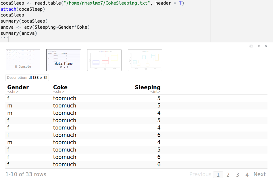
    Gender              Coke              Sleeping
 Length:33          Length:33          Min.   :4.00
 Class :character   Class :character   1st Qu.:5.00
 Mode  :character   Mode  :character   Median :6.00
                                       Mean   :5.97
                                       3rd Qu.:7.00
                                       Max.   :8.00
            Df Sum Sq Mean Sq F value   Pr(>F)
Gender       1  7.120   7.120   9.513  0.00467 **
Coke         2 21.948  10.974  14.662 4.89e-05 ***
Gender:Coke  2  5.693   2.847   3.803  0.03505 *
Residuals   27 20.208   0.748
---
Signif. codes:  0 ‘***’ 0.001 ‘**’ 0.01 ‘*’ 0.05 ‘.’ 0.1 ‘ ’ 1
From the ANOVA table above, we can conclude that both independent variables “Coke consumption” and “Gender” are statistically significant, as well as their interaction. Futhermore, Coke consumption is the most significant factor variable.
library("ggpubr")
ggboxplot(cocaSleep, x = "Coke", y = "Sleeping", color = "Gender",
          palette = c("red", "blue"))
Create a boxplot: x = “Coke” is the name of the x variable, y = “Sleeping” is the name of the y variable, and we change outline colors by groups (color = “gender”) and use custom color palette ( palette = c(“red”, “blue”) ).
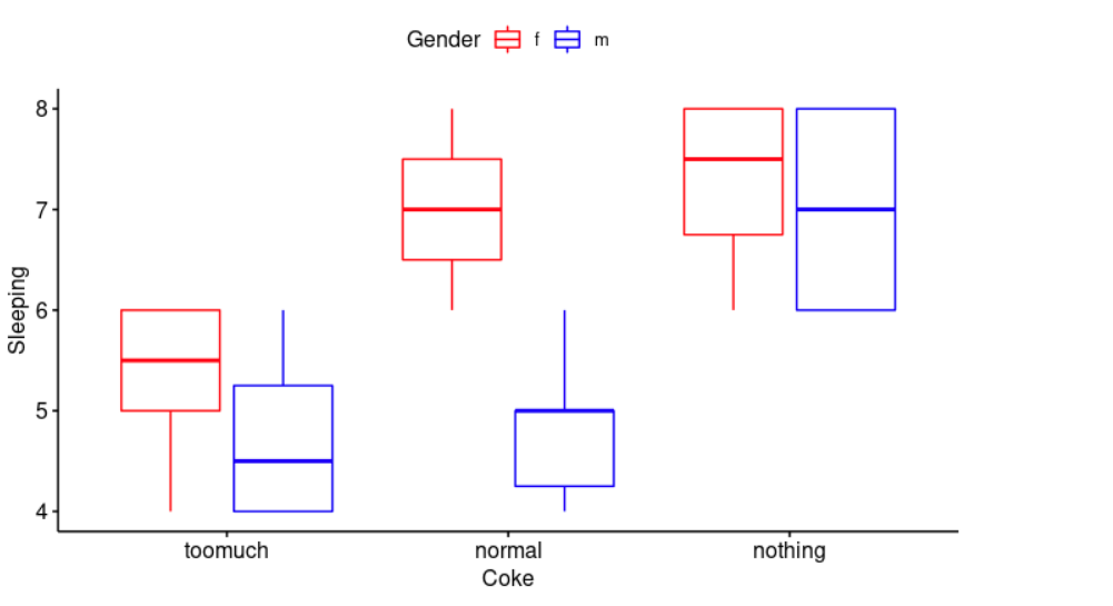
>>> tapply(Sleeping, list(Gender, Coke), mean)
# computes the mean for each factor variable (Gender and Coke) in a vector (Sleeping)
   normal nothing toomuch
f 7.000000    7.25   5.375
m 4.833333    7.00   4.750
>>> tapply(Sleeping, list(Gender, Coke), sd)
     normal   nothing   toomuch
f 0.8164966 0.9574271 0.7440238
m 0.7527727 1.1547005 0.9574271
Caffeine can have a disruptive effect on your sleep. Sodas are “loaded with caffeine and lots of sugar. The caffeine can make it hard to fall asleep, and the sugar may affect your ability to stay asleep”, sleepeducation.org. This data confirm our assumption, but it also indicates that gender plays a role, it is worse in men.
>>> TukeyHSD(anova, which = "Coke")
  Tukey multiple comparisons of means
    95% family-wise confidence level

Fit: aov(formula = Sleeping ~ Gender * Coke)

$Coke
                      diff        lwr         upr     p adj
nothing-normal   1.1611481  0.1972612  2.12503488 0.0158381
toomuch-normal  -0.9538269 -1.8125255 -0.09512825 0.0272046
toomuch-nothing -2.1149749 -3.0940420 -1.13590787 0.0000340
As we can see from the output below, all pairwise comparisons are significant with an adjusted p-value < 0.05. However, it is also revealed a more significant difference between drinking too much Coke or not at all.
plot(anova, 1) # A "residuals versus fits plot" is a scatter plot of residuals on the y axis and fitted values (estimated responses) on the x axis. It is used to detect non-linearity, unequal error variances, and outliers.
library(car)
leveneTest(Sleeping~Gender*Coke)
> leveneTest(Sleeping~Gender*Coke)
Levene's Test for Homogeneity of Variance (center = median)
      Df F value Pr(>F)
group  5  0.7188 0.6149
      27
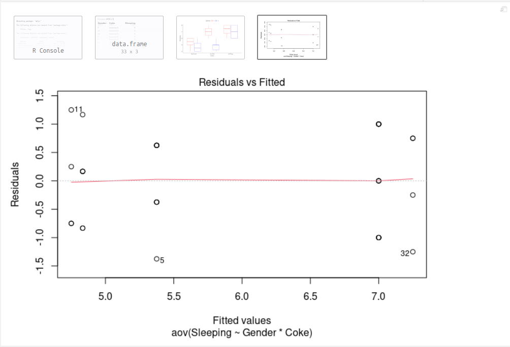
The residuals bounce randomly around the 0 line. Points 5 (f toomuch 5), 11 (f toomuch 6) and 32 (m nothing 8) are detected as outliers, you may need to consider to remove them from your study. Furthermore, we can see that the Levene’s p-value (0.6149) is greater than the significance level of 0.05. In other words, there is no evidence to suggest that the variance across groups is statistically significantly different and we can assume the homogeneity of variances in the different groups.
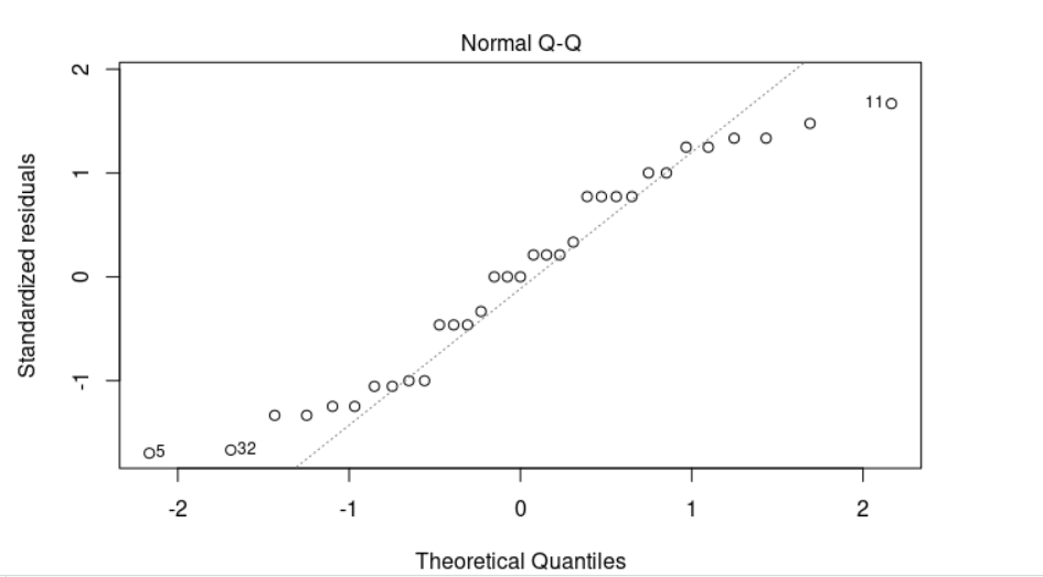
>>> plot(anova, 2)
A “normal probability plot of the residuals” is a way of learning whether it is reasonable to assume that the error terms are normally distributed. If the data follow a normal distribution, then a plot of the theoretical percentiles of the normal distribution versus the observed sample percentiles (the percentiles of the residuals) should be approximately linear.
# Extract the residuals
>>> my_residuals <- residuals(object = anova)
# Run Shapiro-Wilk test
>>> shapiro.test(x = my_residuals ) # The Shapiro–Wilk test is a test of normality in statistics. W = 0.93722, p-value = 0.05641 indicates that normality is not violated.

	Shapiro-Wilk normality test

data:  my_residuals
W = 0.93722, p-value = 0.05641
A one-way repeated measures ANOVA or a within-subjects ANOVA is the equivalent of the one-way ANOVA, but for related, not independent groups. It requires one independent categorical variable and one dependent variable. It is used to compare three or more group means where the participants are the same in each group.
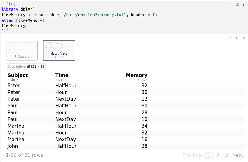
For example, we are going to use a repeated measures ANOVA to understand whether there is a difference in memory retention (subjects are given a list of words that they need to memorize for a test) over time (half an hour, an hour, and next day). In this example, “memory” is the dependent variable (the number of words being remembered by our subjects), whilst the independent variable is “time” (i.e., with three related groups, where each of the three time points is considered a “related group”).
Subject Time Memory
Peter HalfHour 32
Peter Hour 30
Peter NextDay 12
Paul HalfHour 30
Paul Hour 28
Paul NextDay 10
Martha HalfHour 34
Martha Hour 32
Martha NextDay 16
John HalfHour 28
John Hour 24
John NextDay 8
Esther HalfHour 28
Esther Hour 20
Esther NextDay 4
Bew HalfHour 38
Bew Hour 34
Bew NextDay 22
Robert HalfHour 32
Robert Hour 30
Robert NextDay 12 \
myData <- timeMemory %>% group_by(Time) # group_by() takes an existing data frame and converts it into a grouped one (time is the grouping variable) where operations are performed "by group"
get_summary_stats(myData, type = "mean_sd") # get_summary_stats computes summary statistics for myData. type is the type of summary statistics, eg., "full", "common", "mean_sd", etc.
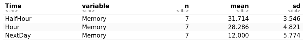
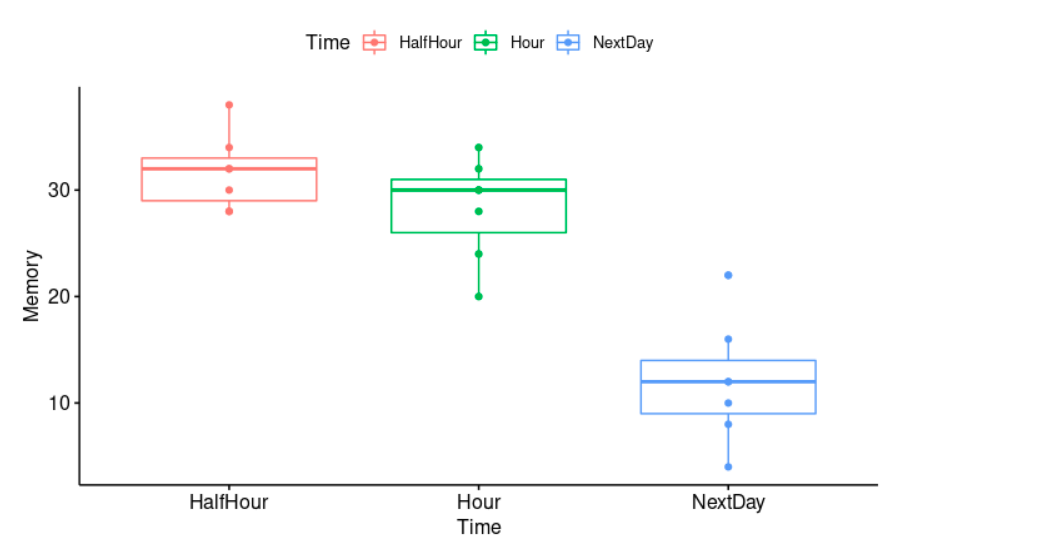
Obviously, the passing of time has a negative effect on memory. The longer the time from learning to testing, the less material (number of words) will be remembered.
library(rstatix)
identify_outliers(myData, Memory) #takes a data frame and extract rows suspected as outliers
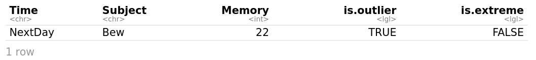
There is no extreme outliers, but Bew NextDay 22 is detected as an outlier. 22 seems to be a lot of words being remembered after twenty four hours compared with other subjects results.
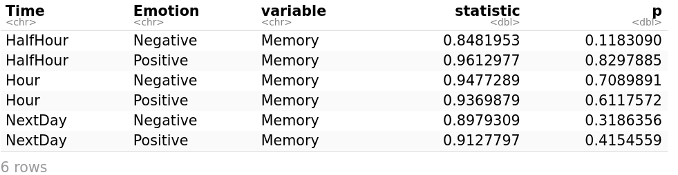
shapiro_test(myData, Memory)
The Shapiro–Wilk test is a test of normality in statistics. The Memory is normally distributed at each time point (HalfHour, Hour, and NextDay), as it is shown by the Shapiro-Wilk’s test because all probabilities are greater than 0.05 (p > 0.05). 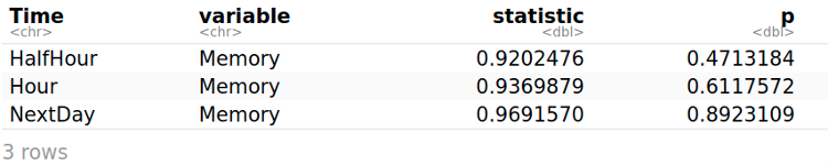
ggqqplot(myData, "Memory", facet.by = "Time", color="Time")
We draw a “quantile-quantile” plot to visually check the normality assumption using ggqqplot: myData (the data frame), facet.by (it specifies the grouping variable, “Time”), and color (point color). If the data is normally distributed, the points in the QQ-normal plot lie on a straight diagonal line. 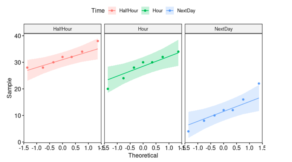
$ANOVA
  Effect DFn DFd   F        p p<.05   ges
1   Time   2  12 302 5.47e-11     * 0.789
$`Mauchly's Test for Sphericity`
  Effect     W     p p<.05
1   Time 0.976 0.942
The assumption of sphericity is automatically checked during the ANOVA test. The null hypothesis is that the variances of the differences between groups are equal. Therefore, a significant p-value indicates that the variances of group differences are not equal, and a not significant p-value (p = 0.942 > 0.05) indicates that we can assume sphericity.
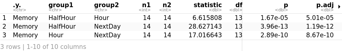
The Memory is statistically significantly different at the different time points: F(2, 12) = 302, p = 5.47e-11 < .05.
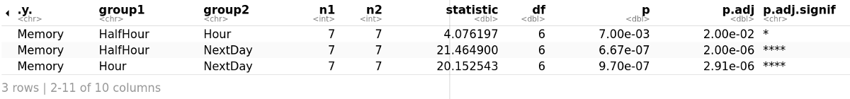
Considering the Bonferroni adjusted p-value (p.adj), it can be seen that the effect of time in memory is statistically significant at each time point. It is less statistically significant after just half an hour which makes a lot of sense as half an hour is not much time.
It is used when there are two factors in the experiment and the same subjects take part in all of the conditions of the experiment. We evaluate simultaneously the effect of two within-subject factors and their interaction on a dependent variable.
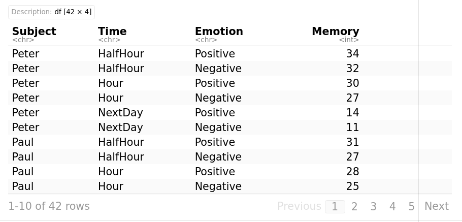
Suppose we have a slightly different experiment in which there are two independent variables: time of day at which subjects are tested (with three levels: half an hour, an hour, and next day) and emotional reaction to words (with two levels: positive and negative). Subjects are given a memory test under all permutations of these two variables. A two-way repeated-measures ANOVA is an appropriate test in these circumstances.
Subject Time Emotion Memory
Peter HalfHour Positive 34 | Peter HalfHour Negative 32
Peter Hour Positive 30 | Peter Hour Negative 27
Peter NextDay Positive 14 | Peter NextDay Negative 11
Paul HalfHour Positive 31 | Paul HalfHour Negative 27
Paul Hour Positive 28 | Paul Hour Negative 25
Paul NextDay Positive 14 | Paul NextDay Negative 9
Martha HalfHour Positive 34 | Martha HalfHour Negative 31
Martha Hour Positive 32 | Martha Hour Negative 31
Martha NextDay Positive 16 | Martha NextDay Negative 9
John HalfHour Positive 29 | John HalfHour Negative 27
John Hour Positive 24 | John Hour Negative 21
John NextDay Positive 12 | John NextDay Negative 7
Esther HalfHour Positive 28 | Esther HalfHour Negative 27
Esther Hour Positive 20 | Esther Hour Negative 19
Esther NextDay Positive 10 | Esther NextDay Negative 7
Bew HalfHour Positive 38 | Bew HalfHour Negative 37
Bew Hour Positive 34 | Bew Hour Negative 32
Bew NextDay Positive 22 | Bew NextDay Negative 12
Robert HalfHour Positive 32 | Robert HalfHour Negative 31
Robert Hour Positive 30 | Robert Hour Negative 28
Robert NextDay Positive 15 | Robert NextDay Negative 9
myData <- timeMemory %>% group_by(Time, Emotion)
# group_by() takes an existing data frame and converts it into a grouped one (Time and Emotion are the grouping variables) where operations are performed "by group"
get_summary_stats(myData, type = "mean_sd") # get_summary_stats computes summary statistics for myData. type is the type of summary statistics, eg., "full", "common", "mean_sd", etc.
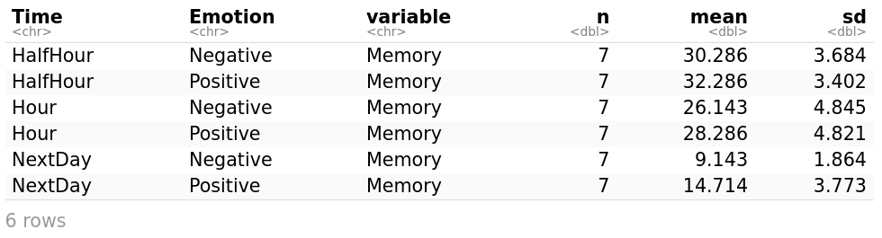
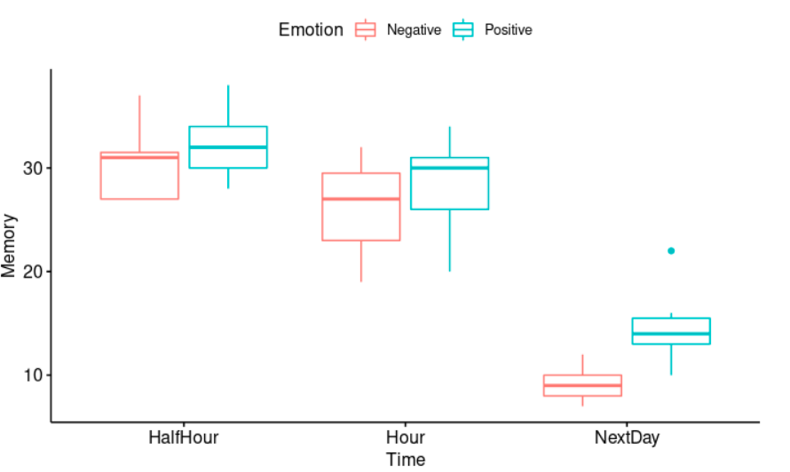
Obviously, the passing of time has a negative effect on memory. The longer the time from learning to testing, the less material (number of words) will be remembered. Besides, positive emotional words are typically processed and remembered more accurately and efficiently than neutral or negative words.
library(rstatix)
identify_outliers(myData, Memory)
#takes a data frame and extract rows suspected as outliers

There is no extreme outliers, but Bew Positive NextDay 22 is detected as an outlier. 22 seems to be a lot of positive words being remembered after twenty four hours compared with other subjects.
ggqqplot(myData, "Memory", color="Time") + facet_grid("Time ~ Emotion")
We draw a “quantile-quantile” plot to visually check the normality assumption using ggqqplot. With face_grid we can split our plot into many plots. Its syntax is as follows: facet_grid(row_variable ~ column_variable). If the data is normally distributed, the points in the QQ-normal plot lie on a straight diagonal line. 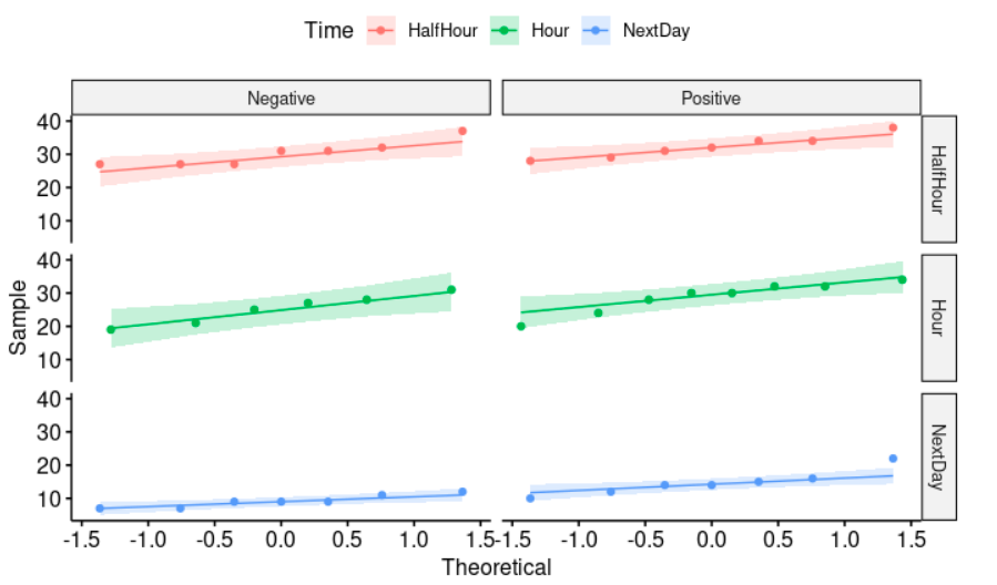
ANOVA Table (type III tests)

$ANOVA
        Effect DFn DFd       F        p p<.05   ges
1         Time   2  12 324.037 3.61e-11     * 0.844
2      Emotion   1   6  91.263 7.51e-05     * 0.170
3 Time:Emotion   2  12  10.073 3.00e-03     * 0.051
The Memory is statistically significantly different at the different time points (F(2, 12) = 324.037, p < 0.05) and under both emotional words conditions (F(1, 6) = 91.263, p < 0.05). There is also a statistically significant two-way interaction between Time and Emotion (F(2, 12) = 10.073, p < 0.05). In other words, the impact that one factor (e.g., time) has on the outcome or dependent variable (Memory) depends on the other factor (Emotion) and vice versa.
Considering the Bonferroni adjusted p-value (p.adj), it can be seen that the effect of time in memory is statistically significant at each time point.
“The binomial distribution with parameters n and p is the discrete probability distribution of the number of successes in a sequence of n independent experiments, each asking a yes-no question, and each with its own Boolean-valued outcome: success (with probability p) or failure (with probability q = 1 − p),” (Wikipedia, Binomial distribution).
A binomial test compares a sample proportion to a hypothesized proportion. The test has the following null and alternative hypotheses: H0: π = p, the population proportion π is equal to some value p. Ha: π ≠ p, the population proportion π is not equal to some value p.
Binomial tests are used in situations where a researcher wants to know whether or not a subject is just guessing or truly is able to perform some task. For example, a monkey is shown two pictures of dots simultaneously. Then, it is shown two choices: the previous dots added together and a different number. Let’s suppose that the experiment is repeated 100 times and the monkey ended up selecting the right answer on 68 of the trials. 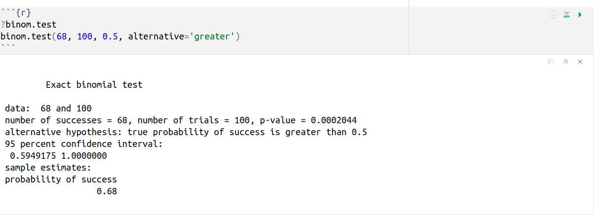
binom.test(68, 100, 0.5, alternative=‘greater’) performs an exact test of a simple null hypothesis about the probability of success in a Bernoulli experiment where: x = 68 is the number of successes; n = 100 is the number of trials; p = 0.5 is the hypothesized probability of success; and alternative=‘greater’ indicates the alternative hypothesis.
The binomial test tells us something about what flipping a coin could have done (p = 0.5). It states that the binomial process, flipping a coin p=1/2, is capable of producing 65/100 or greater with only a very small probability (0.0002044). Therefore, the monkey is not really good at Maths, but it is very unlikely that the 68% correct answers could be explained by pure chance, so it was not just guessing. Hire the fucking monkey!
In other words, p-value is less than 0.05. It indicates strong evidence against the null hypothesis. Therefore, we reject the null hypothesis, and accept the alternative hypothesis: the true probability of success is greater than 0.5.
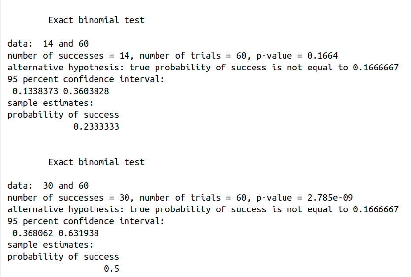
How can we distinguish the fair from the loaded dice? binom.test(14, 60, 1/6), so x = 14 is the number of successes of an outcome, e.g., the die landing with a six; n = 60 is the number of trials; and p = 1/6 is the hypothesized probability of success (a fair dice).
p-value = 0.1664, it is higher than 0.05 (> 0.05), so it is not statistically significant. It indicates strong evidence for the null hypothesis. This means that we retain the null hypothesis, p = 1/6, the dice is fair.
binom.test(30, 60, 1/6), so x = 30, the die has landed with a six 30 times; n = 60 is the number of trials; and p = 1/6 is the hypothesized probability of success (a fair dice).
p-value = 2.785e-09, it is lower than 0.05 (> 0.05), so it is statistically significant. It indicates strong evidence against the null hypothesis. This means that the dice is loaded. In other words, it is very unlikely that a fair dice will land on six 30 times out of 60.

JustToThePoint Copyright © 2011 - 2024 Anawim. ALL RIGHTS RESERVED. Bilingual e-books, articles, and videos to help your child and your entire family succeed, develop a healthy lifestyle, and have a lot of fun. Social Issues, Join us.
This website uses cookies to improve your navigation experience.
By continuing, you are consenting to our use of cookies, in accordance with our Cookies Policy and Website Terms and Conditions of use.


