Polynomials, Equations, and Systems of equations

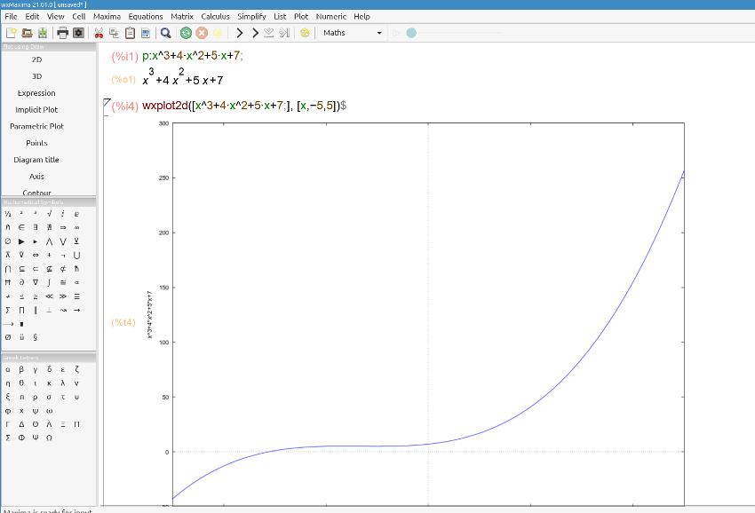
A polynomial is an expression consisting of variables or indeterminates and coefficients, that involves only the operations of addition, subtraction, multiplication, and non-negative integer exponentiation of variables. If there’s a single indeterminate x, a polynomial can always be rewritten as a_nxⁿ + a_n-1x^n-1 + a_n-2x^n-2 + … + a₁x + a₀.

• Let’s work with polynomials using wxMaxima. Maxima is the program that does the actual mathematics and wxMaxima is just a graphical user-friendly interface. Define a polynomial, p: x^3 + 4*x^2 + 5*x+ 7; Observe that xⁿ is written as x^n.
• Let’s plot it: Plot, Plot2D… or type wxplot2d ([x^3 + 4*x^2 + 5*x + 7], [x, -5, 5]); Observe Maxima’s plotting command: plot2d (expr, range_x, options), where expr is an expression that depends on only one variable, or the name of a function. range_x is a list with three elements, the first one being the name of the variable and the other two elements define the minimum and maximum values.
• If we want to substitute the variable x in our polynomial by a given value (e.g. 1), the command subst is used: subst(1, x, p); You can also type: p, x=1;

Fundamental polynomial operations

• First, we define the polynomials p y q: p: x^3 + 2*x^2 + 5; q: 3*x^2 + 5*x + 7;
• Let’s add (p + q) and subtract them (p - q). The most important thing is to look for and combine like terms present in the two polynomials. Like terms are terms whose variables and exponents are the same, eg. 2*x² + 3*x² = 5*x², 2*x² - 3*x² = -x²
• p + 2*q; returns x^3 + 2*(3*x^2 + 5*x +7) + 2*x^2 + 5. Select the Simplify Expression option from the Simplify menu or type ratsimp(%) to simplify our last polynomial expression.
• To multiply two polynomials (p*q): multiply each term of one polynomial by every term of the other; add those answers and combine all of the like terms (5*x⁴ + 6*x⁴ = 11*x⁴). p*q = x³*q + 2*x²*q + 5q = 3*x⁵ + 5*x⁴ + 7*x³ + 6*x⁴ + 10*x³ + 14*x² + 15*x² + 25*x + 35 = 3*x⁵ +11*x⁴ +17*x³ + 29*x² + 25*x + 35.

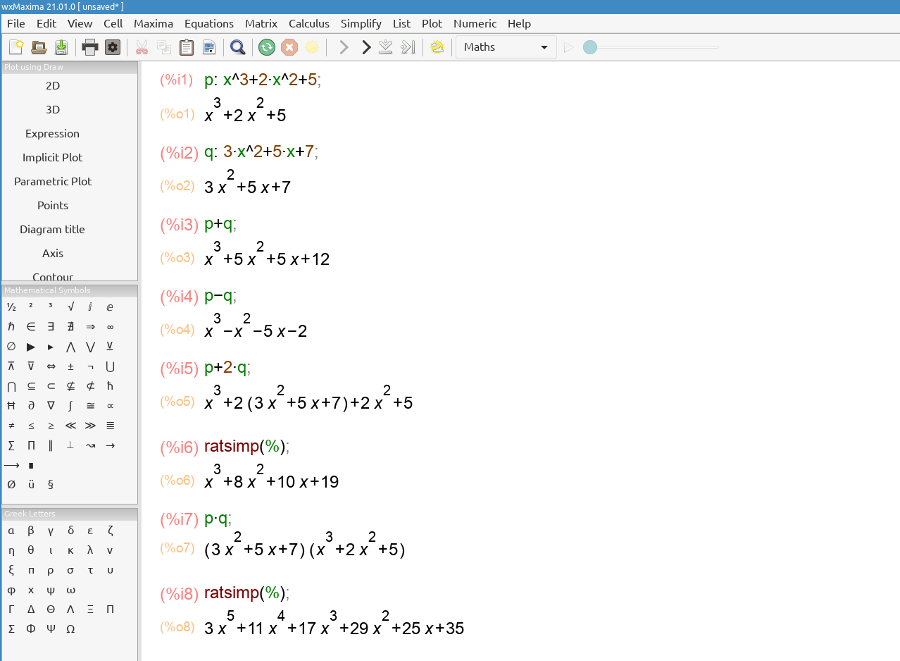
Remember that when you multiply two terms you must multiply the coefficients and add the exponents, e.g. 2*x² * 5*x³ = 10*x⁵;

• The examples so far have been limited to expressions containing one variable, such as p: x^3 + 2*x^2 + 5; q: 3*x^2 + 5*x + 7; but polynomials can also contain multiple variables or indeterminates. ratsimp((3*x-4*y) * (5*x-2*y)); returns 8*y² -26*x*y + 15*x². expand((2*x + 3*y)*(3*x + 4*y + 7)); = 12*y² + 17*x*y + 21*y + 6*x² +14*x. The Maxima’s command expand() expands an expression completely.
• Let’s divide two polynomials: Calculus, Divide Polynomials or simply type: divide(p, q); It returns the quotient and remainder of the polynomial p divided by the polynomial q, [(3*x+1) ⁄ 9, -(26*x-38) ⁄ 9]. We know that dividend (p) = divisor (q) × quotient + remainder, so ratsimp(q * (3*x+1) ⁄ 9 -(26*x-38) ⁄ 9); returns p.
• We can extract the coefficients of a polynomial: coeff (3*b^3*a^4 + 2*b^2*a^2 + 4*b*a + 1, a^4); returns the a^4 coefficient, 3*b^3. bothcoeff (3*b^3*a^4 + 2*b^2*a^2 + 4*b*a + 1, a^4); returns the a^4 coefficient and the remaining terms, [3*b^3, 2*a^2*b^2 + 4*a*b +1]. Besides, hipow (y^3 * x^2 + x * y^4, x); returns the highest power or exponent of x, 2.

Factorization of a Polynomial

• Factorization is the breaking apart of a polynomial P(x) into a product of its factors: factor(6*x^4 -12*x^3 +4*x^2); returns 2*x^2* (3*x^2 -6*x + 2). 2*x² and 3*x² -6*x + 2 are irreducible polynomials.
• factor(x^4-16); returns (x-2) * (x+2) * (x^2 + 4). It is quite simple, we change the variable x^2=t, so x^4 -16 turns into t^2 -16. factor (t^2 -16); = (t-4)(t+4). Thus, x^2=4 (x = 2, x = -2) and x^2=-4.
• More examples: factor(x^4 -6*x^3 +5*x^2 +24*x -36); = (x-3)^2 * (x-2) * (x+2). factor(2*x^4+x^3-8*x^2-x+6); = (x-1) * (x+1) * (x+2) * (2*x-3)

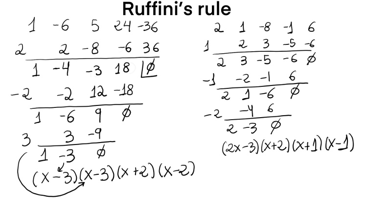
In general, if you want to factorize a polynomial, you may need to extract a common factor, e.g., x^2 + x = x(x + 1), 6*x^4 -12*x^3 +4*x^2 = 2*x^2* (3*x^2 -6*x + 2), use remarkable formulas, e.g., 25*x^2 -49 = (5*x)^2-(7)^2=(5*x-7)(5*x+7) as we are using (a+b)(a-b)=a² -b² or divide the polynomial between (x-a) by Ruffini method.

Roots of a Polynomial

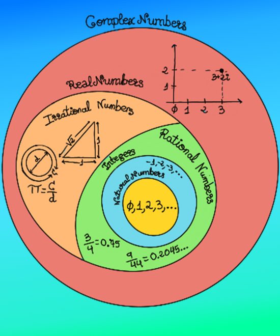
The roots or zeroes of a polynomial are those values of the variable that cause the polynomial to evaluate to zero. In other words, the root of a polynomial p(x) is that value “a” that p(a) = 0.

• solve(x^4 -6*x^3 +5*x^2 +24*x -36); returns [x = -2, x = 2, x = 3] As shown below, the roots of a polynomial are those values of the variable that cause the polynomial to evaluate to zero, so they are the values where its graph crosses the x-axis.

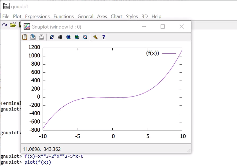
Gnuplot is a free, command-driven, interactive plotting program. The set grid command allows grid lines to be drawn on the plot. The set xzeroaxis command draws a line at y = 0. set xrange [-5:5] and set yrange [-60:40] set the horizontal and vertical ranges that will be displayed. plot and splot are the primary commands in Gnuplot, e.g., plot sin(x)/x, splot sin(x*y/20), or plot [-5:5] x**4 -6*x**3 +5*x**2 +24*x -36, where x**4 is x⁴ and -6*x**3 is -6*x³.

• solve(2*x^4 + x^3 -8*x^2 -x +6); = [x=-2, x=-1, x=1, x=3⁄2]

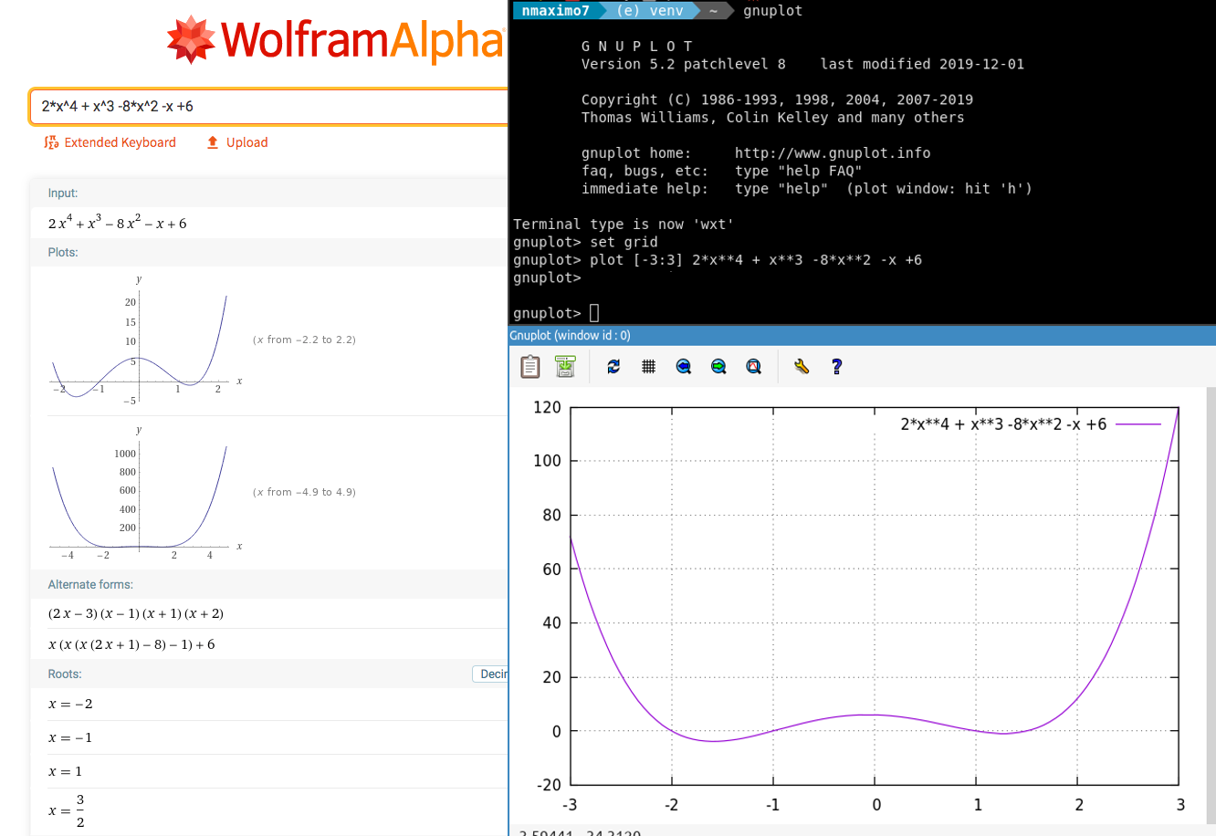
WolframAlpha is a great tool for finding polynomial roots. It also factors polynomials and plots them.

• solve(x^4-16); it finds all the real and complex roots of x⁴ -16 = [x = 2 %i, x = -2, x = -2 %i, x = 2] = ("%i" means i) [x = 2i, x = -2, x = -2i, x = 2]

Roots and factorization of a Polynomial with Python

vim factor.py

>>> import sympy
>>> x = sympy.Symbol('x') # SymPy variables are objects of the Symbol class.
>>> polynomial = x**4 -6*x**3 +5*x**2 +24*x -36 # polynomial = x4 -6*x3 +5*x2 +24*x -36
>>> print(sympy.solve(polynomial)) # sympy.solve algebraically solves equations and polynomials. The roots of polynomial are 
[-2, 2, 3]
>>> print(sympy.factor(polynomial)) # sympy.factor takes a polynomial and factors it into irreducible factors 
(x - 3)**2*(x - 2)*(x + 2)
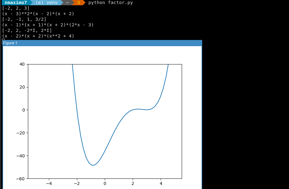
>>> polynomial2 = 2*x**4+x**3-8*x**2-x+6
>>> print(sympy.solve(polynomial2))
[-2, -1, 1, 3/2]
>>> print(sympy.factor(polynomial2))
(x - 1)*(x + 1)*(x + 2)*(2*x - 3)
>>> polynomial3 = x**4-16
>>> print(sympy.solve(polynomial3))
[-2, 2, -2*I, 2*I]
>>> print(sympy.factor(polynomial3))
(x - 2)*(x + 2)*(x**2 + 4)

import numpy as np # NumPy is a library for array computing with Python
import matplotlib.pyplot as plt # Matplotlib is a plotting library for the Python programming language 
X = np.linspace(-5, 5, 50, endpoint=True) # Return evenly spaced numbers over the interval [-5, 5] as the values on the x axis.
def p(x):
        return x**4 -6*x**3 +5*x**2 +24*x -36 # This is the polynomial that we are going to plot. 
F = p(X) # The corresponding values on the y axis are stored in F.
plt.ylim([-60, 40]) # Set the y-limits on the current axes.
plt.plot(X, F) # These values are plotted using the mathlib's plot() function.
plt.show() # The graphical representation is displayed by using the show() function.

First-degree equations

An algebraic equation will always have an equal “=” sign and at least one unknown number or quantity, called a variable, represented by a letter (x, y, or z). Some examples of equations are 7*x = 12, 2*x + 6 = 8, x² + 4*x + 4 = 0, etc. Solving an equation means finding the value of the unknown number, quantity or variable. The degree of an equation is the highest exponent to which the unknown or unknows are elevated.

• A first degree equation is a polynomial equation whose degree or maximum exponential numerical value of the unknown or unknowns is 1. In other words, each term is either a constant or a product of a constant and one variable. For example, 2*x + 6 = x + 4. We define the equation: eq: 2*x + 6 = x + 4; and ask Maxima to solve it: solve(eq);. It returns [x = -2].

Let’s solve the equation: A. Relocate terms: Move the terms that carry the variable “x” to the left and the numbers that do not carry “x” to the right: 2*x -x = 4 -6. Notice that a term may be moved from one member of an equation to the other member (side) provided the sign of the term is changed. B. Now simplify (or collect) the like terms: x = -2.

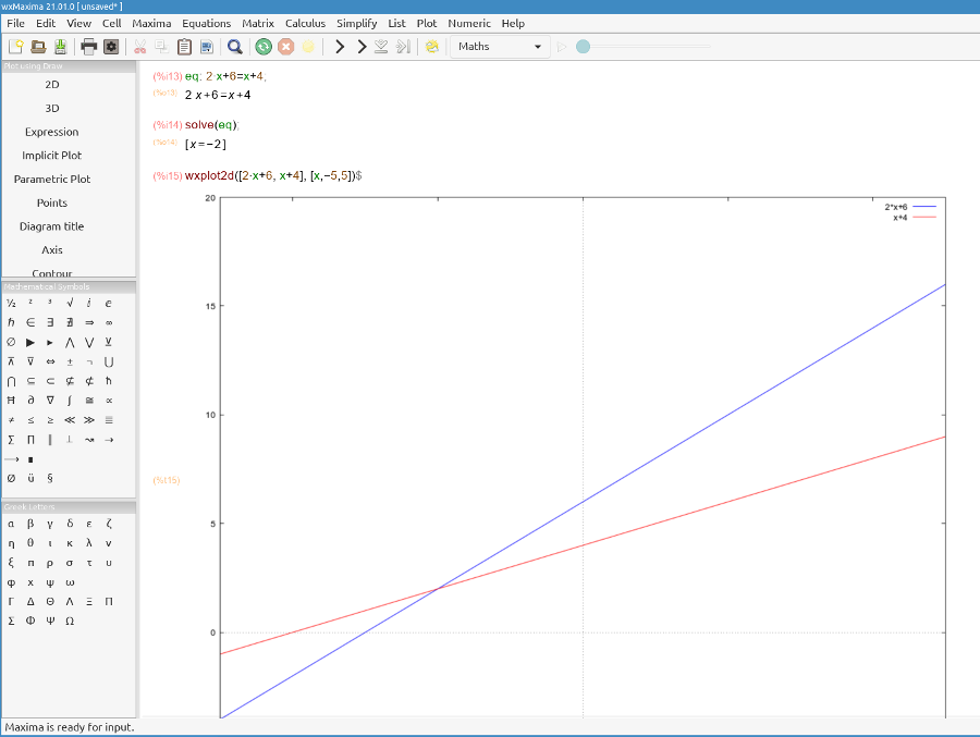
Graphically, 2*x + 6 and x + 4 are two lines that intersect in x = -2.

• Let’s see another example. eq: x +1 -3*x = 4 -3*x +6 +x; and ask Maxima to solve it: solve(eq); Maxima returns [] It means that it does not have a solution.

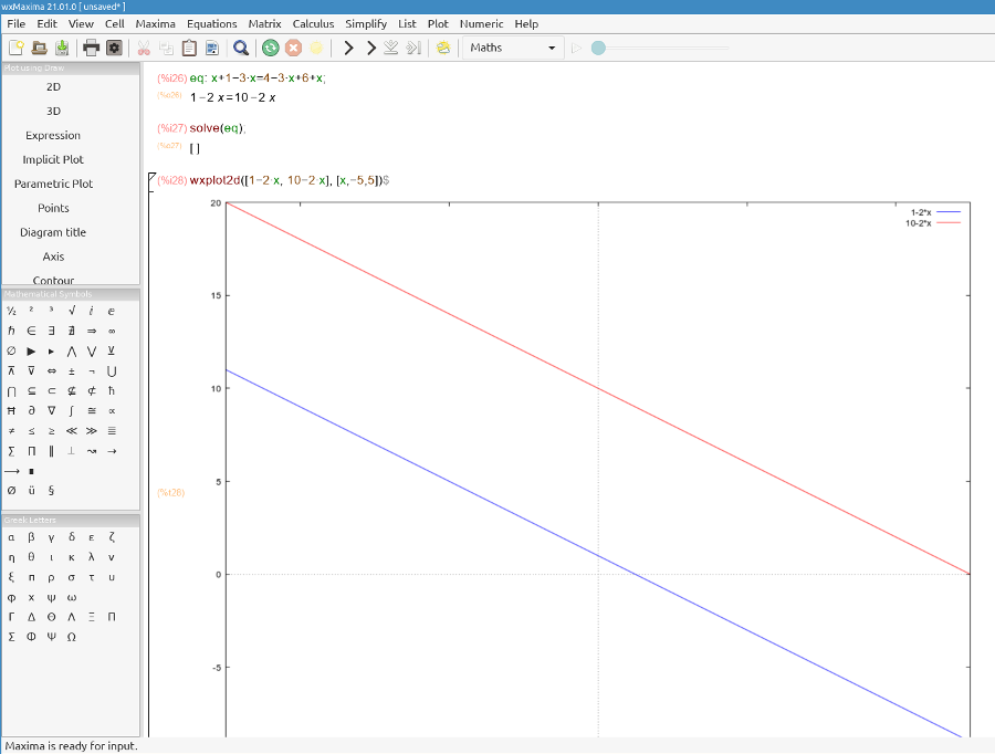
A. Relocate terms: x -3*x +3*x -x = 4 + 6 - 1. B. Simplify: 0 = 9. The equation does not have a solution. It is an impossible equation. Graphically, 1 - 2*x, 10 -2*x are two parallel lines that do not intersect, and thus, there are no solutions.

• Finally, eq: x + 4 -3*x = 1 -3*x +x +3; solve(eq); returns all. A. Relocate terms: x -3*x +3*x -x = 1 + 3 -4. B. Simplify: 0 = 0. Any number is therefore solution of this equation. Here is an equation that admits an infinity of solutions. The graphical representation shows that there are not two lines, but a single one.

Second-degree equations

Quadratic or second-degree equations are those where the greatest exponent to which the unknown is raised is the exponent 2.

• Let’s define the equation eq: x^2 -5*x +6 = 0; and ask Maxima to solve it solve(eq); and plot it wxplot2d([x^2 -5*x +6], [x,-5,5]); We are plotting it in gnuplot, too.

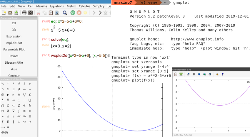
The solution is: x = ^{-b ± √b2 -4*a*c}⁄_2*a = ^{5 ± √52 -4*1*6}⁄_2*1 = ^{5 ± √25 -24}⁄₂ = ^{5 ± 1}⁄₂. Solutions = 3, 2. expand((x-3)*(x-2)); returns x^2 -5*x +6 and its graph is a parabola. Its two roots (2, 3) are the x-intercepts of the graph (those value of x where the graph crosses or touches the x-axis).

• Another example is: eq: x^2 -8*x +16 = 0; Next, we ask Maxima to solve it (solve(eq);) and plot it: wxplot2d([x^2 -8*x +16], [x,-1,6]); We are going to type the same equation in WolframAlpha, too. Obviously, we get the same results with both applications.

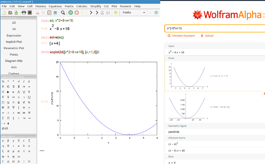
The solution is: x = ^{-b ± √b2 -4*a*c}⁄_2*a = ^{8 ± √82 -4*1*16}⁄_2*1 = ^{8 ± √64 -64}⁄₂ = ^{8 ± 0}⁄₂. It is a double root: 4. expand((x-4)*(x-4)); returns x^2 -8*x +16 and its graph is also a parabola, but the graph does not cross the x-axis, it just touches it at x = 4.

• Finally, we are going to solve a third quadratic equation: eq: x^2+4; solve(eq); returns [x=-2i, x=2i], and plot it: wxplot2d([x^2+4], [x,-5, 5]));

The solution is: x = ^{-b ± √b2 -4*a*c}⁄_2*a = ^{0 ± √02 -4*1*4}⁄_2*1 = ^{± √-16}⁄₂ = ^{± 4i}⁄₂ = ±2i. expand((x-2%i)*(x+2%i)); returns x^2 +4. There are no real roots and the graph does not cross or touch the x-axis. Its graph tells us that the roots of the equation are complex numbers.

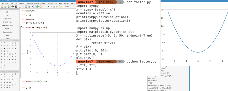
>>> import sympy # Let's solve it in Python using SymPy
>>> x = sympy.Symbol('x')  # SymPy variables are objects of the Symbol class.
>>> equation = x**2 +4 # Define the equation x2 + 4
>>> print(sympy.solve(equation)) # sympy.solve algebraically solves equations and polynomials. The roots of the equation are: 
[-2*I, 2*I]
>>> print(sympy.factor(equation)) # We ask Python to factor our equation (x-2i)(x+2i), but fails.

import numpy as np  # NumPy is a library for array computing with Python
import matplotlib.pyplot as plt # Matplotlib is a plotting library for Python
X = np.linspace(-5, 5, 50, endpoint=True) # Return evenly spaced numbers over the interval [-5, 5] as the values on the x axis.
def p(x):
	return x**2+4 # This is the equation that we are going to plot. 
F = p(X) # The corresponding values on the y axis are stored in F.
plt.ylim([0, 30]) # Set the y-limits on the current axes.
plt.plot(X, F) # These values are plotted using the mathlib's plot() function.
plt.show() # The graphical representation is displayed by using the show() function.

Systems of equations in two variables

A system of linear equations consists of two or more equations made up of two or more variables such that all equations are considered simultaneously. A system of equations in two variables consists or comprises of two linear equations of the form
a*x + b*y = c
d*x + e*y = f
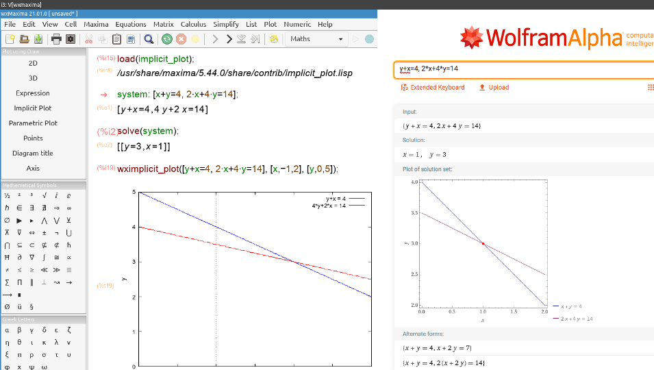
The solution to a system of linear equations in two variables is any ordered pair (x, y) that satisfies each equation independently, the point at which the lines representing the linear equations intersect.

• Suppose there is a nice farm with chicken and rabbits. Together there are 4 heads and 14 legs. How many chickens does the farm have? How many rabbits?
• We can make a couple of equations out of the given information. We know that the statement “there are four heads” means there are four animals, chickens and rabbits, altogether. We also know from general knowledge that rabbits have four legs and chickens have two. Therefore, let’s assume that X is the number of chickens and Y is the number of rabbits. The problem can be rewritten as…
• So there are one chicken and three rabbits. Let’s ask Maxima and WolfranAlpha to solve it. We define system as the system of equations in two variables: system: [x+y=4, 2x+4y=14]; and use the command solve(system); to find its solution. Finally, we plot it using wximplicit_plot. Observe that the implicit_plot package needs to be loaded before this command can be used: load(implicit_plot);

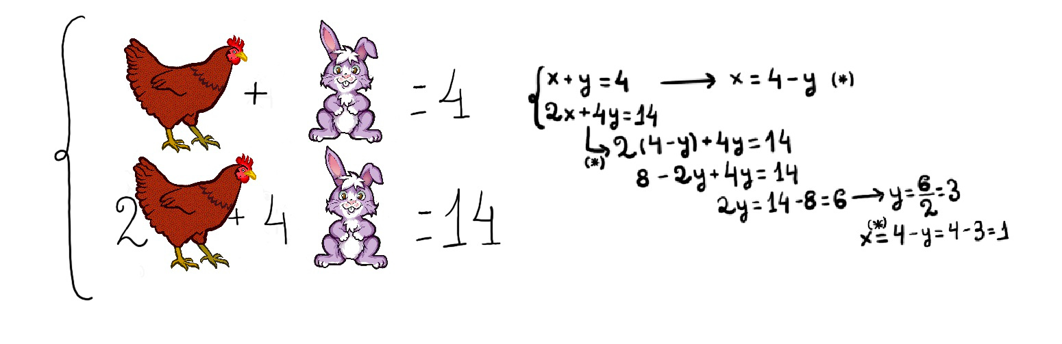
In a system of linear equations, each equation corresponds with a line. This is a determined compatible system with one solution pair (3, 1). This is the point where the two lines (the straight lines are secant) intersect.

• Next, we do another system of equations: 3*x +2*y = 7, 8*x -6*y = -4. This is also a determined compatible system with one solution pair (1, 2).
• Let’s solve the system of equations: 3*x+2*y=7, 9*x+6*y=21. This is an undetermined compatible system. It has infinite solutions and its lines are coincident.

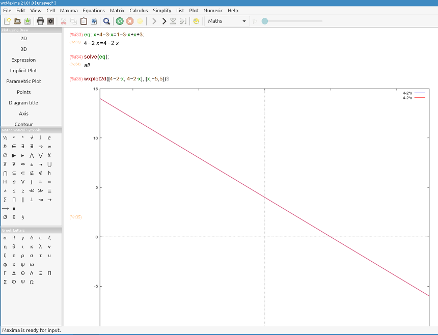
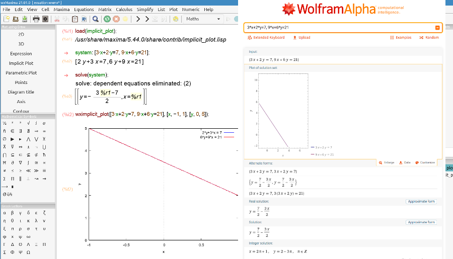
The two lines are the same line indeed, so every coordinate pair on the line is a solution to both equations: (1, 2), (3, -1), etc. Equations in a dependent system can be derived from one another; they describe the same line, so 9*x + 6*y = 21 is basically the same than 3*x + 2*y=7. It is the result of multiplying both sides of the equation by 3.

• Finally, we are going to solve this system of equations: 3*x + 2*y = 7, 6*x + 4*y = 15. This is an incompatible or inconsistent system. It has no solution. The two lines are parallel and they do not intersect.

user@pc:~$ python
Python 3.8.6 (default, May 27 2021, 13:28:02) 
[GCC 10.2.0] on linux
Type "help", "copyright", "credits" or "license" for more information.
>>> import sympy 
>>> x = sympy.Symbol('x')
>>> y = sympy.Symbol('y')
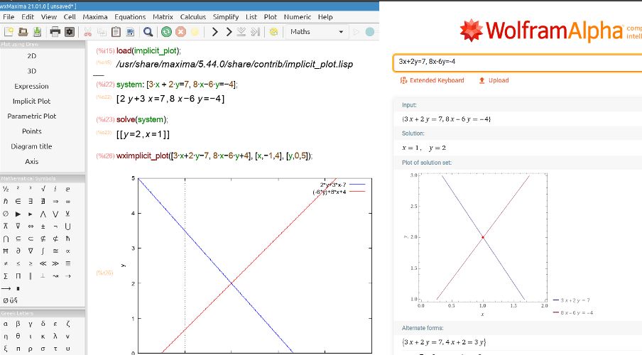
>>> sympy.solve([3*x+2*y-7, 8*x-6*y+4])
{x: 1, y: 2}
>>> sympy.solve([3*x+2*y-7, 9*x+6*y-21])
{x: 7/3 - 2*y/3}
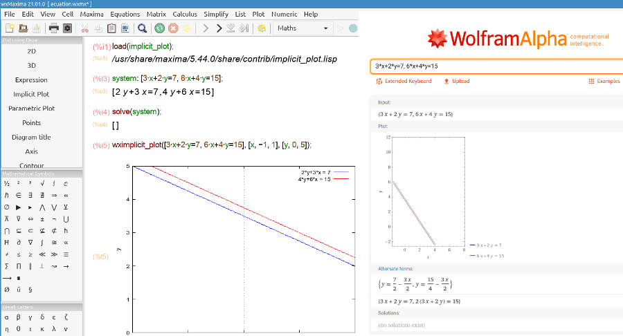
>>> sympy.solve([3*x+2*y-7, 6*x+4*y-15])
[]

Solving inequalities

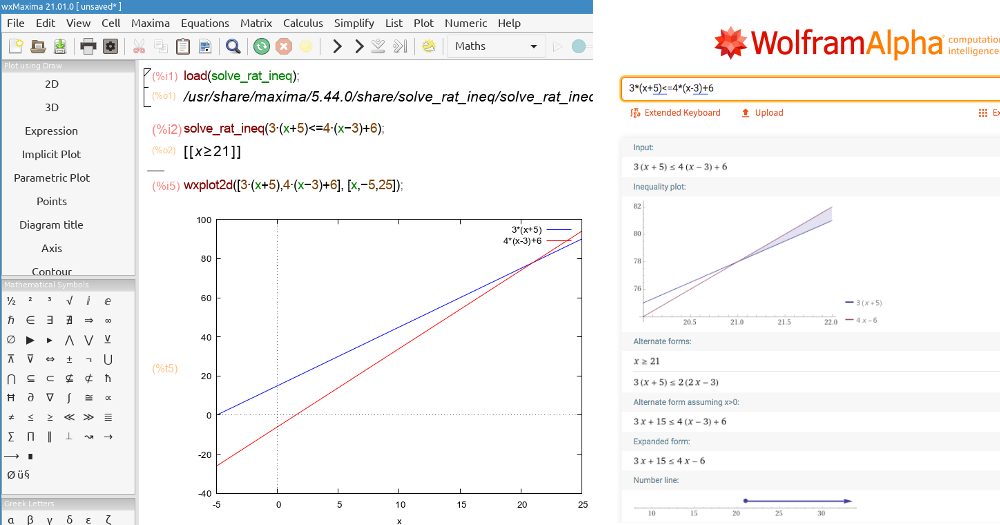
An inequality is a relation that makes a non-equal comparison between two numbers or mathematical expressions, e.g., -3*x-7<2*x-5, 5*y-2>14, etc.

• Let’s solve this inequality: 3*(x+5) <= 4*(x-3) + 6. A. We rearrange or relocate terms in the same way as we do with equations: 3*x+3*5 <= 4*x -4*3 +6. 3*x-4*x <= -12 + 6 -15. B. Simplify the like terms: -x <= -21. C. However, there is a big difference, multiplying both sides by a negative number (-1) does change the direction of the inequality: x ≥ 21.
• You solve simple rational inequalities in Maxima by using the solve_rat_ineq command: solve_rat_ineq( 3*(x+5) <= 4*(x-3) + 6 );. Previously, you will need to load the package solve_rat_ineq: load(“solve_rat_ineq”);
• A more difficulty inequality is: x^2 <= 7*x -10. We use the command: to_poly_solve([S], [x]); To access a function in a package, you must first load it: load(fourier_elim); However, this package is experimental, so WolfranAlpha is recommended. We have also plotted the functions x^2 and 7*x-10 and we can observe that [2, 5] is the solution.

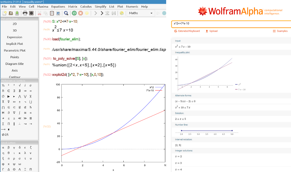
You can always solve the equation x^2 - 7*x -10 = (x-2)(x-5) and prove that x^2 - 7*x -10<= 0 between its roots.
(-∞, 2): x^2 - 7*x -10 > 0;
[2, 5]: x^2 - 7*x -10 <= 0;
(5, -∞): x^2 - 7*x -10 > 0