Vectors, matrices, and system of linear equations

Vectors

A vector is an object that has both a magnitude or size and a direction. “Geometrically, we can picture a vector as a directed line segment, whose length is the magnitude of the vector and with an arrow indicating the direction,” An introduction to vectors", Math Insight.

We are going to use Maxima to work with vectors and matrices.

• First, we define two vectors: v: [3, 4, 5] and w: [2, 7, 1];
• Next, we perform some operations on them. Let’s add both vectors: v+w. Observe that adding the respective components of two vectors yields a vector which is the sum of both vectors. Let u = [u₁, u₂, u₃] and v = [v₁, v₂, v₃]. Then u + v = [u₁+v₁, u₂+v₂, u₃+v₃]. Vector subtraction: u - v = [u₁-v₁, u₂-v₂, u₃-v₃]. Scalar multiplication: 3.v. Multiplying all the components of a vector by a constant is equivalent to multiplying the vector by that constant, k.u = [k*u₁, k*u₂, k*u₃]
• The dot product or scalar product of two vectors is obtained by multiplying their magnitudes with the cosine of the angle between them: u.v=||u|| ||v|| cosθ = u₁*v₁ + u₂*v₂ + u₃*v₃. Thus, v.w = 6 + 28 + 5 = 39.
• The magnitude or Euclidean norm (or Euclidean length) of a vector, denoted by ||v||, is the length of the vector. ||v|| = sqrt(v₁² + v₂² + v₃²) = sqrt(v.v) = sqrt(9 + 16 + 25)= sqrt(50) =sqrt(52 *2) = 5√2.
• Vector cross product in Maxima. vect is a package of functions for vector analysis. We need to load this package: load (“vect”); v~w; calculates the cross product of v and w.
• unitvector(x); returns x/||x||, a unit vector (a vector of length 1) in the same direction as x = [4, 2, 4]/6 (||x|| = sqrt(16 + 4 + 16) = 6) = [2⁄3, 1⁄3, 2⁄3]. Previously, we need to load the eigen package: load(“eigen”);
• rank(matrix(v,w)); = 2. matrix(v, w); returns a matrix with v and w as rows. rank(matrix(v,w)); computes the rank of the matrix(v, w). It is two, so both vectors are independent. Let’s see another example, u: [1, 4, 2]; v: [5, 20, 10]; rank(matrix(u, v)); =1. It is one because u and v are linearly dependent. Observe that v is a scalar multiple of u; in other words, there exists a scalar c = 5 such that v = cu = 5u.

Let’s use Yacas, an easy to use, general purpose Computer Algebra System, a program for symbolic manipulation of mathematical expressions. It is available online, too.

The Ubuntu installation instructions are quite simple: sudo add-apt-repository ppa:teoretyk/yacas, sudo apt-get update, sudo apt-get install yacas

user@pc:~$yacas
This is Yacas version '1.3.6'.
To exit Yacas, enter  Exit(); or quit or Ctrl-c.
Type 'restart' to restart Yacas.
To see example commands, keep typing Example();
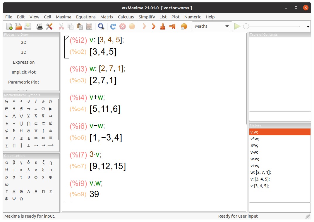
In> v:={3, 4, 5}; # We define two vectors, v and w.
Out> {3,4,5}
In> w:={2, 7, 1};
Out> {2,7,1}
In> v+w; # We perform some operations on them.
Out> {5,11,6}
In> v-w;
Out> {1,-3,4}
In> 3*v;
Out> {9,12,15}
In> v.w; # We ask Yacas for the scalar product of both vectors.
Out> 39
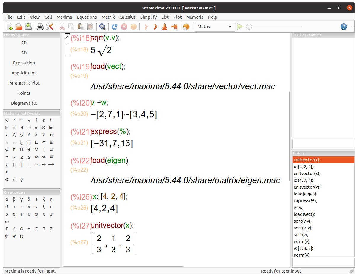
In> sqrt(v.v); # It returns the magnitude of v.
Out> sqrt(50)
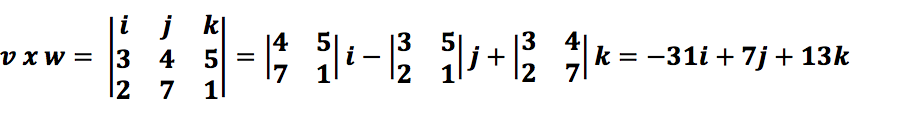
In> CrossProduct(v, w); # It returns the cross product of the vectors v and w.
Out> {-31,7,13}
In> x:={4, 2, 4};
Out> {4,2,4}
In> Normalize(x); # It normalizes a vector. In other words, it returns the normalized (unit) vector parallel to "x", a vector having the same direction as that of a given vector "x" but length or magnitude equal to 1.
Out> {2/3,1/3,2/3}

Let’s work with vectors in Python. You may want to learn much more in our article Vectors in Python.

user@pc:~$ python 
Python 3.8.10 (default, Jun  2 2021, 10:49:15) 
>>> import numpy as np # NumPy is a library that supports vectors and matrices in an optimized way. 
>>> v = np.array([3, 4, 5]) # Data manipulation in Python is almost synonymous with NumPy array manipulation.
>>> w = np.array([2, 7, 1])
>>> np.add(v, w) # numpy.add adds arguments element-wise: v+w.
array([ 5, 11,  6])
>>> np.subtract(v, w) # numpy.subtract subtracts arguments element-wise: v-w.
array([ 1, -3,  4])
>>> v*3
array([ 9, 12, 15])
>>> np.dot(v, w) # It calculates the dot product or scalar product of v and w.
39
>>> np.linalg.norm(v) # It computes the magnitude or Euclidean norm of v.
7.0710678118654755 # = sqrt(50)
>>> np.cross(v, w) # numpy.cross returns the cross product of two vectors. 
array([-31,   7,  13])
>>> x = np.array([4, 2, 4])
>>> x/np.linalg.norm(x) # It normalizes the vector. 
array([0.66666667, 0.33333333, 0.66666667]) # {2/3,1/3,2/3}

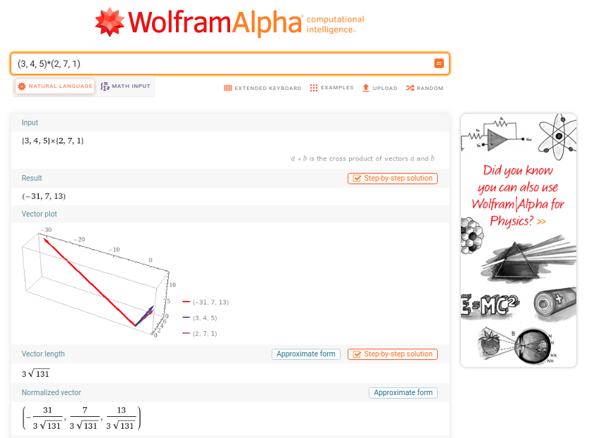
We can use Wolfram Alpha, too. For instance, (3, 4, 5)*(2, 7, 1) or {3, 4, 5}*{2, 7, 1} computes a cross product (it also returns a Vector plot, Vector length, and the Normalized vector); and {3, 4, 5}.{2, 7, 1} computes a dot or scalar product. Besides, we can perform some vector computations: {3, 4, 5} + {2, 7, 1}, {3, 4, 5}-3*{2, 7, 1}; {3, 4, 5}^3;

norm{3, 4, 5} computes the magnitude or norm of a vector; normalize {4, 2, 4} normalizes the vector. Finally, MatrixRank![{3, 4, 5},{2, 7, 1}] = 2. MatrixRank[m] gives the rank of the matrix m and finds the number of linearly independent rows, so {3, 4, 5} and {2, 7, 1} are independent. MatrixRank[{1, 4, 2}, {5, 20, 10}] returns 1 because {1, 4, 2} and {5, 20, 10} are linearly dependent. Vectors in WolframAlpha

Matrices

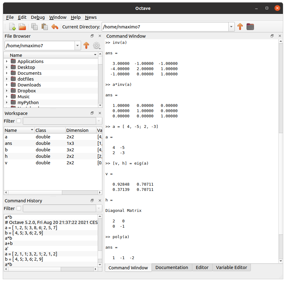
Octave is a program specially designed for manipulating matrices. The easiest way to define matrices in Octave is to type the elements inside square brackets “[]”, each entry could be separated by a comma, and you should replace the commas with semicolons to specify the end of a row, e.g., a = [ 2, 1, 1; 3, 2, 1; 2, 1, 2], b = [ 4, 5; 3, 6; 2, 9]. We can create matrices with random elements, too: b = rand(3, 2).

You can use the standard operators to add (a+b), subtract (a-b), multiply (a*b), power (a^2), and transpose (a’) matrices. The det() function in Octave returns the determinant of a matrix and inv() returns the inverse of a matrix.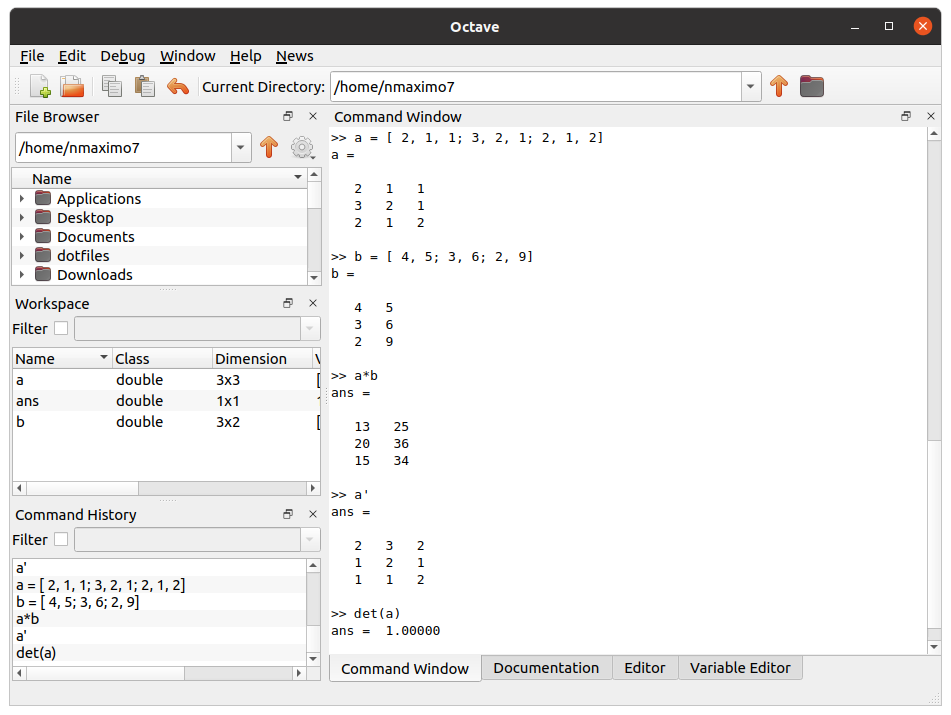

Let’s consider the linear transformation Av = w where A is an “n” by “n” matrix. If v and w are scalar multiples (Av = w = λv), then v is an eigenvector of the linear transformation A and the scale factor λ is the eigenvalue corresponding to that eigenvector.

Av = λv can be stated equivalently as (A -λI)v = 0 where I is the identity matrix, and 0 is the zero vector. This equation has a nonzero solution v if and only if the determinant of the matrix (A -λI) is zero, so the eigenvalues are values λ that satisfy the equation |A - λI| = 0. The left-hand side of this equation is called the characteristic polynomial of A.

Thus, |A - λI| = (λ₁ -λ) (λ₂ -λ)…(λ_n -λ) where λ₁, λ₂, ….λ_n are the eigenvalues of A. In our example, ![v, h]=eig(a) returns the eigenvalues λ₁ = 2 and λ₂=-1, and |A - λI| = (λ₁ -λ) (λ₂ -λ) = (2 -λ)(-1 -λ) = λ₂ -λ -2 (poly(a) returns the characteristic polynomial of a). You can double check: det(a-2*eye(2)) (eye(2) returns a square 2*2 identity matrix) = 0, det(a+eye(2)) = 0, and det(a) = -2 = λ₁*λ₂. Working with matrices in Octave

user@pc:~$yacas # We can obtain the same results with Yacas
This is Yacas version '1.3.6'.
To exit Yacas, enter  Exit(); or quit or Ctrl-c.
Type 'restart' to restart Yacas.
To see example commands, keep typing Example();
In> matrixA := {{1, 2, 5}, {3, 8, 6}, {2, 5, 7}}; # Yacas can manipulate vectors, represented as lists, and matrices, represented as lists of lists. 
Out> {{1,2,5},{3,8,6},{2,5,7}}
In> matrixB := {{3, 4, 5}, {2, 4, 7}, {3, 1, 9}};
Out> {{3,4,5},{2,4,7},{3,1,9}}
In> matrixA + matrixB; # Basic arithmetic operators work on integers, vectors, and matrices.
Out> {{4,6,10},{5,12,13},{5,6,16}}
In> 3*matrixA;
Out> {{3,6,15},{9,24,18},{6,15,21}}
In> Transpose(matrixA); # It gets the transpose of a matrix.
Out> {{1,3,2},{2,8,5},{5,6,7}}
In> Determinant(matrixA); # It returns the determinant of matrixA.
Out> 3
In> Inverse(matrixA); # It gets the inverse of matrixA.
Out> {{26/3,11/3,(-28)/3},{-3,-1,3},{(-1)/3,(-1)/3,2/3}}
In> Trace(matrixA) # It returns the trace of matrixA, the sum of the elements on its diagonal 1 + 8 + 7
Out> 16

Yacas is available online, too. EigenValues(matrix) gets the eigenvalues of a matrix, and CharacteristicEquation(matrix, var) gets the characteristic polynomial of a “matrix” using “var”.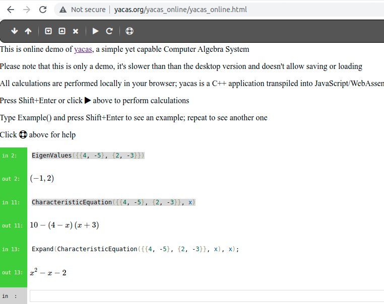

user@pc:~$ python # Let's work with matrices in Python
Python 3.8.10 (default, Jun  2 2021, 10:49:15) 
>>> import numpy as np # NumPy is a library that supports vectors and matrices in an optimized way. 
>>> matrixA=np.array([[1, 2, 5], [3, 8, 6], [2, 5, 7]]) # Data manipulation in Python is almost synonymous with NumPy array manipulation.
>>> matrixB=np.array([[3, 4, 5], [2, 4, 7], [3, 1, 9]])
>>> np.add(matrixA, matrixB) # numpy.add adds arguments element-wise: matrixA + matrixB.
array([[ 4,  6, 10],
       [ 5, 12, 13],
       [ 5,  6, 16]])
>>> np.subtract(matrixA, matrixB) # numpy.subtract subtracts arguments element-wise: matrixA - matrixB.
array([[-2, -2,  0],
       [ 1,  4, -1],
       [-1,  4, -2]])
>>> np.dot(matrixA, matrixB) # If both inputs are 2D arrays, the numpy.dot function performs matrix multiplication.
array([[ 22,  17,  64],
       [ 43,  50, 125],
       [ 37,  35, 108]])
>>> 3*matrixA
array([[ 3,  6, 15],
       [ 9, 24, 18],
       [ 6, 15, 21]])
>>> matrixA.T # We use the T method to transpose a matrix.
array([[1, 3, 2],
       [2, 8, 5],
       [5, 6, 7]])
>>> matrixA.trace() # We use the trace method to calculate the trace of a matrix.
16
>>> np.linalg.matrix_rank(matrixA) # The NumPy's linear algebra linalg.matrix_rank method returns the rank of matrixA.
3
>>> np.linalg.det(matrixA)  # The NumPy's linear algebra det method computes the determinant of matrixA.
3.0000000000000018
>>> np.linalg.inv(matrixA)  # The NumPy's linear algebra inv method calculates the inverse of matrixA.
array([[ 8.66666667,  3.66666667, -9.33333333],
       [-3. , -1. ,  3. ],
       [-0.33333333, -0.33333333,  0.66666667]])
>>> matrix=np.array([[4, -5], [2, -3]])
>>> eigenvalues, eigenvectors = np.linalg.eig(matrix) # Let's calculate the eigenvalues and eigenvectors of a square matrix.
>>> eigenvalues
array([ 2., -1.])
>>> eigenvectors
array([[0.92847669, 0.70710678],
       [0.37139068, 0.70710678]])
>>> np.poly(matrix) # It returns the coefficients of the characteristic polynomial of a matrix.
array([ 1., -1., -2.])

Alternatively, we can work with WolframAlpha. Transpose({{1, 2, 5}, {3, 8, 6}, {2, 5, 7}}) returns the transpose of the matrix {{1, 2, 5}, {3, 8, 6}, {2, 5, 7}}. Det({{1, 2, 5}, {3, 8, 6}, {2, 5, 7}}) calculates the determinant of a matrix (3). Inverse({{1, 2, 5}, {3, 8, 6}, {2, 5, 7}}) gives the inverse of a square matrix.

Observe that the syntax is almost the same as Python, Yacas or Octave, e.g., {{1, 2, 5}, {3, 8, 6}, {2, 5, 7}} * {{1,2,3},{3,2,1},{1,2,3}}, {{1, 2, 5}, {3, 8, 6}, {2, 5, 7}} + {{1,2,3},{3,2,1},{1,2,3}}, Trace{{1, 2, 5}, {3, 8, 6}, {2, 5, 7}} (= 16), Rank{{1, 2, 5}, {3, 8, 6}, {2, 5, 7}} (=3), etc.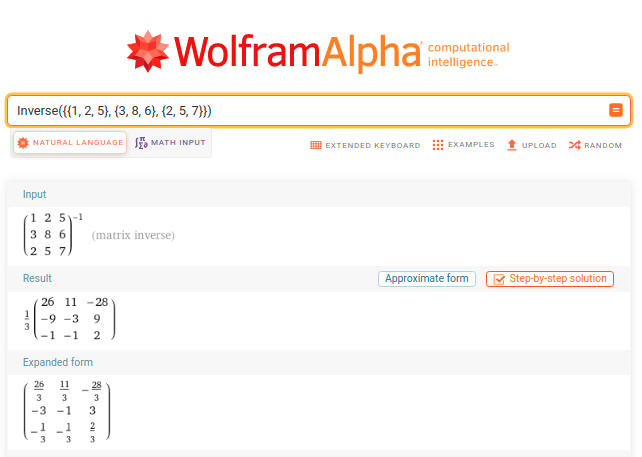

However, you can use plain English to enter your queries in WolframAlpha: find the eigenvalues of the matrix {{4, -5}, {2, -3}} or calculate eigenvalues of the matrix {{4, -5}, {2, -3}}. CharacteristicPolynomial{{4, -5}, {2, -3}} gives the characteristic polynomial for the matrix {{4, -5}, {2, -3}}.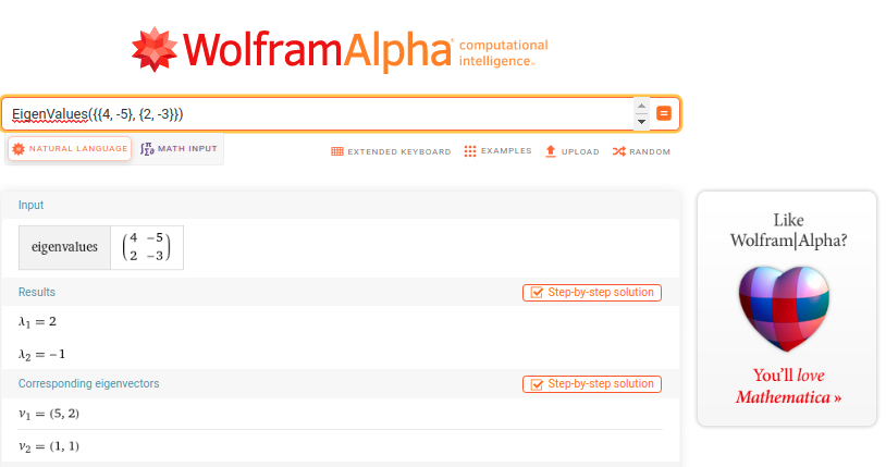

System of linear equations

A system of linear equations (or linear system) is a set or collection of one or more linear equations. Observe that only simple variables are allowed in linear equations, e.g., x², z³, and √x are not allowed. For example, 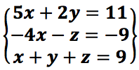A solution of a system of linear equations is a vector or an assignment of values to the variables that is simultaneously a solution of each equation in the system.

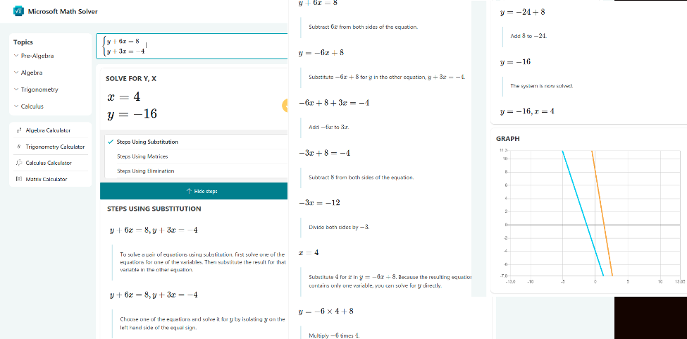
A system of linear equations is consistent if it has at least one solution. Alternatively, a system with no solutions will be called inconsistent. A system of linear equations has either a unique solution (consistent, e.g., y+6x = 8, y+3x = -4; Solution: x = 4, y = -16), infinite solutions (consistent, e.g., 2x+y ​= 4, 6x + 3y= 12; Solutions: y = 4-2x), or no solutions (inconsistent, e.g. 2x+y ​= 4, 6x + 3y= 10).

For any system of linear equations, there are three helpful matrices that are very important: the coefficient matrix containing the coefficients of the variables (A), the augmented matrix which is the coefficient matrix with an extra column added containing the constant terms of the linear system (the coefficients of the variables together with the constant terms) and the constant matrix or the column vector (b) of constant terms. The vector equation is equivalent to a matrix equation of the form Ax = b.

user@pc:~$yacas
This is Yacas version '1.3.6'.
To exit Yacas, enter  Exit(); or quit or Ctrl-c.
Type 'restart' to restart Yacas.
To see example commands, keep typing Example();
In> A:={{6, 1}, {3, 1}} # Define the coefficient matrix. y+6x = 8, y+3x = -4; 
Out> {{6,1},{3,1}}
In> B:={8, -4}  # Define the constant matrix.
Out> {8,-4}
In> MatrixSolve(A, B) # It solves the matrix equation Ax = b.
Out> {4,-16} # It has a unique solution x= 4, y = -16.

Microsoft Math Solver provides free step by step solutions to a variety of Math problems.

user@pc:~$yacas
In> A:={{5, 2, 0}, {-4, 0, -1}, {1, 1, 1}} # Define the coefficient matrix.
Out> {{5,2,0},{-4,0,-1},{1,1,1}}
In> B:={11,-9, 9} # Define the constant matrix.
Out> {11,-9,9}
In> MatrixSolve(A, B) # It solves the matrix equation Ax = b.
Out> {1,3,5}

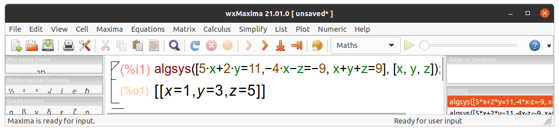
Wolfram Alpha is more than capable of solving systems of linear equations: 5*x+2*y=11, -4*x-z=-9, x+y+z=9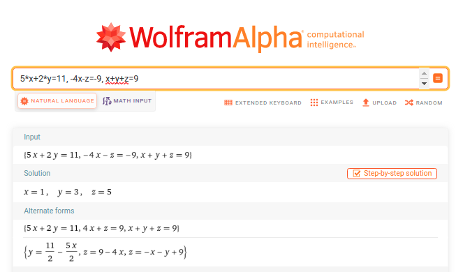

Maxima’s command algsys (![expr_1, …, expr_m], [x_1, …, x_n]) solves the simultaneous polynomial equations expr_1, …, expr_m for the variables x_1, …, x_n, e.g., algsys([5*x+2*y=11,-4*x-z=-9, x+y+z=9], [x, y, z]); Solve a system of equations using Maxima

The Rouché–Capelli theorem determines the number of solutions for a system of linear equations. The necessary and sufficient condition for a system of m equations and n unknowns to have a solution is that the rank of its coefficient matrix (r) and that of its augmented matrix are equal (r’).

If r= rang(A) ≠r’= rang(A|b) the system is incompatible. If r = r’=n the system is a determinate compatible system; in other words, it has only one solution. If r = r’ ≠ n the system is an indeterminate compatible system, it has infinite solutions.

user@pc:~$ python # Let's solve system of linear equations in Python
Python 3.8.10 (default, Jun  2 2021, 10:49:15) 
>>> import numpy as np # NumPy is a library that supports vectors and matrices in an optimized way. 
>>> matrixA=np.array([[5, 2, 0], [-4, 0, -1], [1, 1, 1]]) # Data manipulation in Python is almost synonymous with NumPy array manipulation. We define the coefficient matrix ...
>>> vectorB=np.array([11, -9, 9]) # ... and the constant matrix.
>>> np.linalg.solve(matrixA, vectorB) # It solves a linear matrix equation or a system of linear equations.
array([1., 3., 5.])
>>> np.linalg.matrix_rank(matrixA) # The NumPy's linear algebra linalg.matrix_rank method returns the rank of matrixA.
3
>>> matrixExtended = np.column_stack([matrixA, vectorB]) # numpy.column_stack staks 1-D arrays (our constant matrix) as columns into a 2-D array (our coefficient matrix) so we can get the  augmented matrix A|b.
>>> matrixExtended
array([[ 5,  2,  0, 11],
       [-4,  0, -1, -9],
       [ 1,  1,  1,  9]])
>>> np.linalg.matrix_rank(matrixExtended) # Observe that rang(A) = rang(A|b) = 3 (r=r'=n) so our system is a determinate compatible system, it has an unique solution, [1, 3, 5].
3

Let’s solve a second system of linear equations. 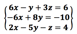Easy peasy lemon squeezy with Wolfram Alpha:

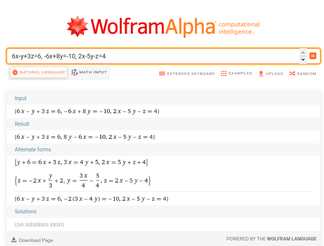
Oops, it does not find any solutions. Let’s see with Maxima what’s the problem.

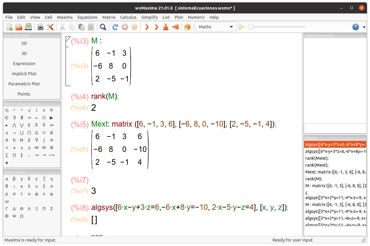
Observe that algsys([6*x-y+3*z=6,-6*x+8*y=-10, 2*x-5*y-z=4], [x, y, z]); returns [] because rank(Mext) = rank ( matrix ([6, -1, 3, 6], [-6, 8, 0, -10], [2, -5, -1, 4]) ) = 3 ≠ 2 = rank(M) = rank ( matrix ([6, -1, 3], [-6, 8, 0], [2, -5, -1]); ). In conclusion, rang(A) ≠ rang(A|b) so the system is incompatible.

Let’s see a third system of linear equations:

user@pc:~$yacas
This is Yacas version '1.3.6'.
To exit Yacas, enter  Exit(); or quit or Ctrl-c.
Type 'restart' to restart Yacas.
To see example commands, keep typing Example();
In> A:={{8, 1, 4}, {5, -2, 4}, {1, 1, 0}} # Define the coefficient matrix.
Out> {{8,1,4},{5,-2,4},{1,1,0}}
In> B:={9,6, 1} # Define the constant matrix.
Out> {9,6,1}
In> MatrixSolve(A, B) # It tries to solve the matrix equation Ax = b, but fails.
Out> {0,Undefined,Undefined}

Maxima shows that r = r’= 2 ≠ n = 3, the system is an indeterminate compatible system, it has infinite solutions. Solutions: x = ^-(4t-8)⁄₇, y = ^4t-1⁄₇, z = t.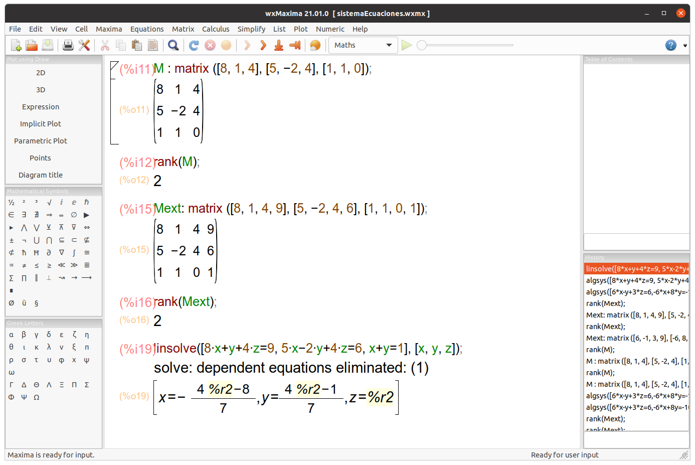

user@pc:~$ python # Let's solve system of linear equations in Python
Python 3.8.10 (default, Jun  2 2021, 10:49:15) 
>>> import numpy as np # NumPy is a library that supports vectors and matrices in an optimized way. 
>>> matrixA=np.array([[8, 1, 4], [5, -2, 4], [1, 1, 0]]) # Data manipulation in Python is almost synonymous with NumPy array manipulation. We define the coefficient matrix ...
>>> vectorB=np.array([9, 6, 1]) # ... and the constant matrix.
>>> np.linalg.matrix_rank(matrixA)  # The NumPy's linear algebra linalg.matrix_rank method returns the rank of matrixA.
2
>>> matrixExtended = np.column_stack([matrixA, vectorB]) # column_stack staks 1-D arrays (our constant matrix) as columns into a 2-D array (our coefficient matrix) so we can get the augmented matrix A|b.
>>> matrixExtended
array([[ 8,  1,  4,  9],
       [ 5, -2,  4,  6],
       [ 1,  1,  0,  1]])
>>> np.linalg.matrix_rank(matrixExtended)
2 # It shows that r = r'= 2 ≠ n = 3, the system is an **indeterminate** compatible system, it has _infinite solutions_.
>>> np.linalg.lstsq(matrixA, vectorB, rcond=None) # Calling linalg.solve(matrixA, vectorB) requires that matrixA is a square and full-rank matrix. In other words, all its rows must be linearly independent and its determinant could not be zero. Otherwise, it will raise the exception: LinAlgError: Singular matrix.
(array([0.88888889, 0.11111111, 0.44444444]), array([], dtype=float64), 2, array([1.09823822e+01, 2.71795522e+00, 2.54972035e-16]))

np.linalg.lstsq gives us one of the solutions, 0.88888889, 0.11111111, 0.44444444. This result is consistent with what we obtained in Maxima: z = 0.44444444, x = -(40.44444444-8)/7 = 0.88888889142, y = -(40.44444444-1)/7 = 0.11111110857.