Mathematical analysis

Limits

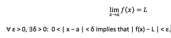
A limit is the value to which a function grows close as the input approaches some value. One would say that the limit of f, as x approaches a, is L. Formally, for every real ε > 0, there exists a real δ > 0 such that for all real x, 0 < | x − a | < δ implies that | f(x) − L | < ε. In other words, f(x) gets closer and closer to L as x moves closer and closer to a.

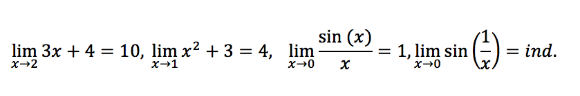
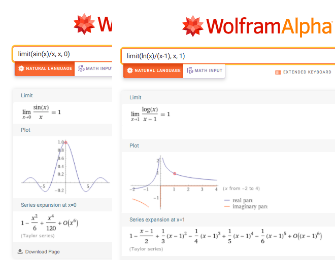
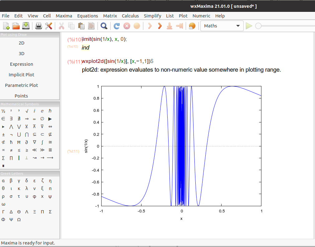
To compute a limit in (a cross-platform graphical front-end for the computer algebra system Maxima), we use the command limit with the following syntax: limit(f(x), x, a). Some examples are: limit(3*x+4, x, 2); returns 10; limit(x^2+3, x, 1); returns 4; limit(sin(x)/x, x, 0); returns 1. Limits in Maxima

sin(¹⁄_x) wobbles between -1 and 1 an infinite number of times between zero and any positive x value, no matter how small or close to zero, that’s why there is not limit for sin(¹⁄_x) as x approaches zero.

WolframAlpha provides functionality to evaluate limits, too. Observe that the function x*sin(¹⁄_x) is a somewhat different story from sin(¹⁄_x). Since -1 ≤ sin(¹⁄_x) ≤ 1, -x ≤ x * sin(¹⁄_x) ≤ x, then as x approaches zero so must x * sin(¹⁄_x).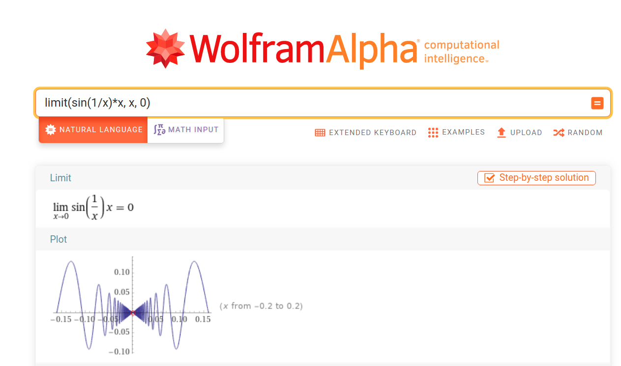

Write in WolframAlpha, limit(sqrt(x), x, infinite), limit(1/x, x, infinite), and limit(1/x, x, 0). You can also compute one-sided limits from a specified direction: lim 1/x as x->0+.

A one-sided limit is the limit of a function f(x) as x approaches a specified value or point “a” either from the left or from the right.

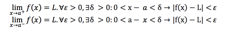
The minus sign indicates “from the left”, and the plus sign indicates “from the right”. In other words, f(x) gets closer and closer to L as x moves closer and closer to “a” from the left or from the right.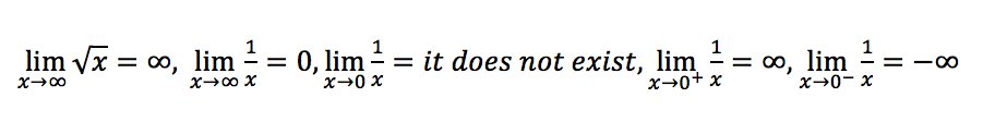

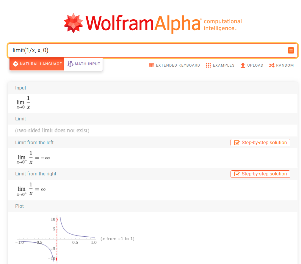
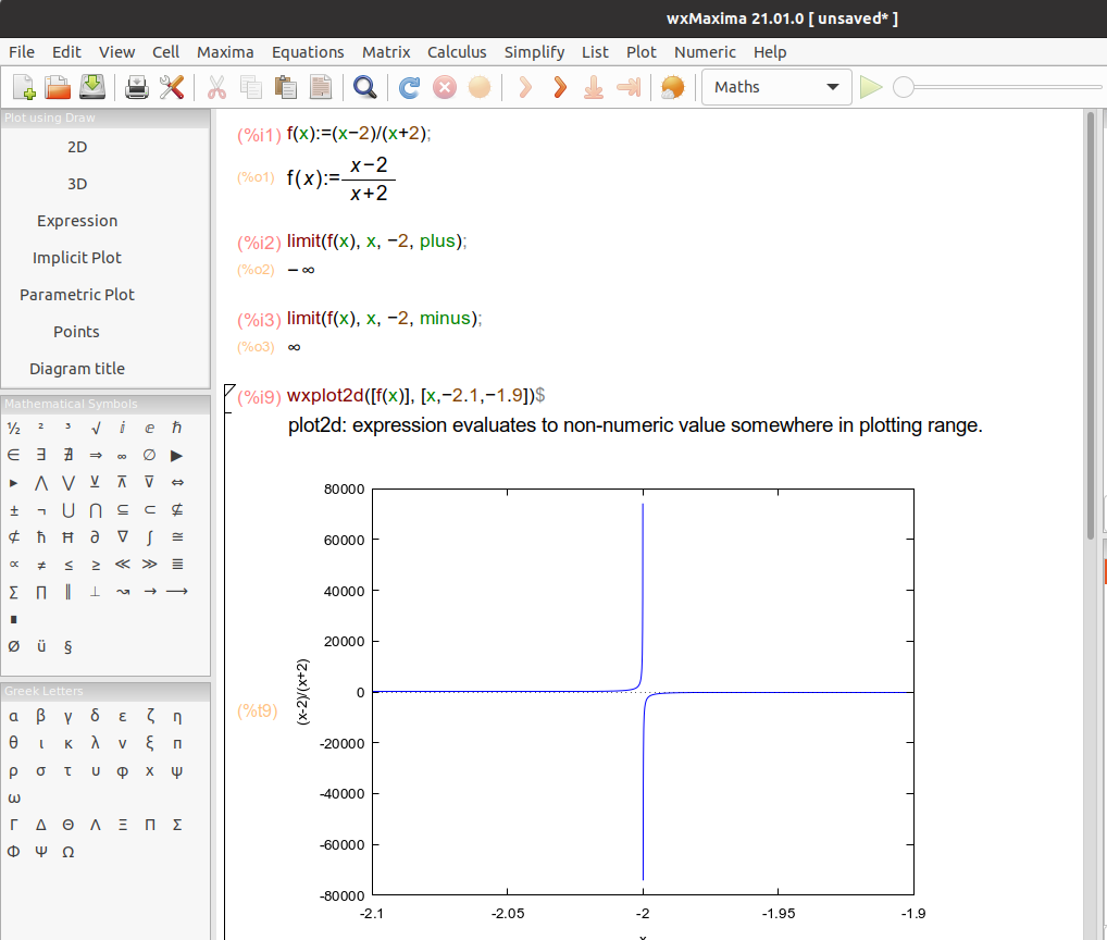
Please consider that we do not take ¹⁄₀ as ∞ or −∞. Division by zero is undefined. Similarly, the limit of ¹⁄_x as x approaches 0 is also undefined. However, if you take the limit of ¹⁄_x as x approaches zero from the left or from the right, you get negative and positive infinity respectively. These limits are not equal and that’s why the limit of ¹⁄_x as x approaches 0 is undefined.

x = 0 is a vertical asymptote of ¹⁄_x. In general, if the limit of the function f(x) is ±∞ as x→a from the left or the right, x = a is a vertical asymptote of the graph of the function y = f(x).

We can use Python to calculate limits, too. We will use SymPy, “a Python library for symbolic mathematics. It aims to become a full-featured computer algebra system (CAS) while keeping the code as simple as possible in order to be comprehensible and easily extensible.”

user@pc:~$ python
Python 3.8.10 (default, Jun  2 2021, 10:49:15) 
[GCC 10.3.0] on linux
Type "help", "copyright", "credits" or "license" for more information.
>>> from sympy import * # Import the SymPy library
>>> x = symbols('x')
>>> limit(sin(x), x, 0) # SymPy can compute limits with the limit function. Its syntax is limit(f(x), x, a).
0
>>> limit(x**2, x, 0)
0
>>> limit(sqrt(x), x, oo) # Infinite is written as oo, a double lowercase letter 'o'.
oo # A function has an infinite limit if it either increases or decreases without bound.
>>> limit(1/x, x, 0, '+') # Limit has a fourth argument, dir, which specifies a direction.
oo
>>> limit(1/x, x, 0, '-')
-oo
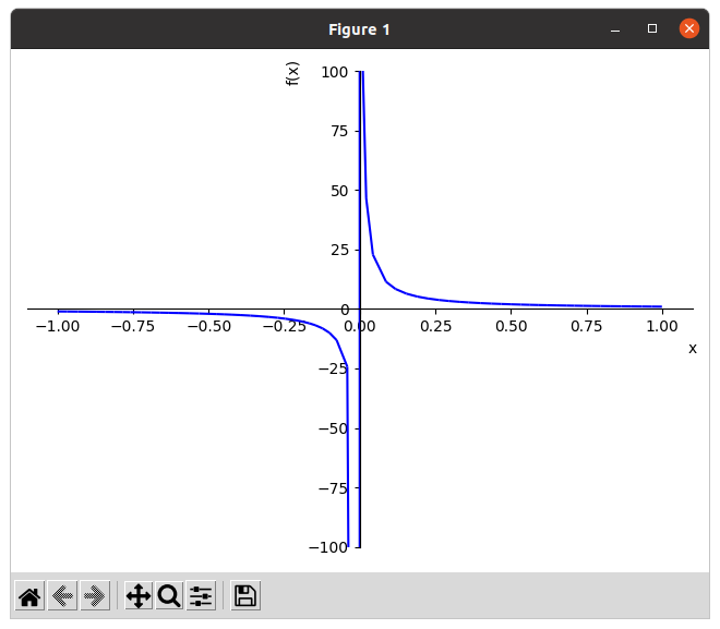
>>> from sympy.plotting import plot # The plotting module allows you to make 2-dimensional and 3-dimensional plots.
>>> plot(1/x, (x, -1, 1), ylim= (-100, 100), line_color = 'blue') # It plots 1⁄x. ylim denotes the y-axis limits and line_color specifies the color for the plot. 

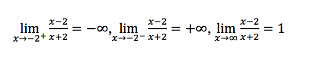
Maxima computes the limit of expr (limit (expr, x, a, dir)) as x approaches “a” from the direction dir. dir may have the value “plus” for a limit from above or right, “minus” for a limit from below or left, or may be omitted. You may also want to try f(x):= ^(x-2)⁄_(x+2); limit(f(x), x, infinity); It will return 1.

y = 1 is a horizontal asymptote of ^(x-2)⁄_(x+2). In general, if the limit of the function f(x) is “a” as x→±∞, y = a is a horizontal asymptote of the graph of the function y = f(x).

Let’s see a last example, f(x) = ^{x2 +2*x -2}⁄_{x²+3*x +7}. y = 1 is a horizontal asymptote of ^{x2 +2*x -2}⁄_{x²+3*x +7}.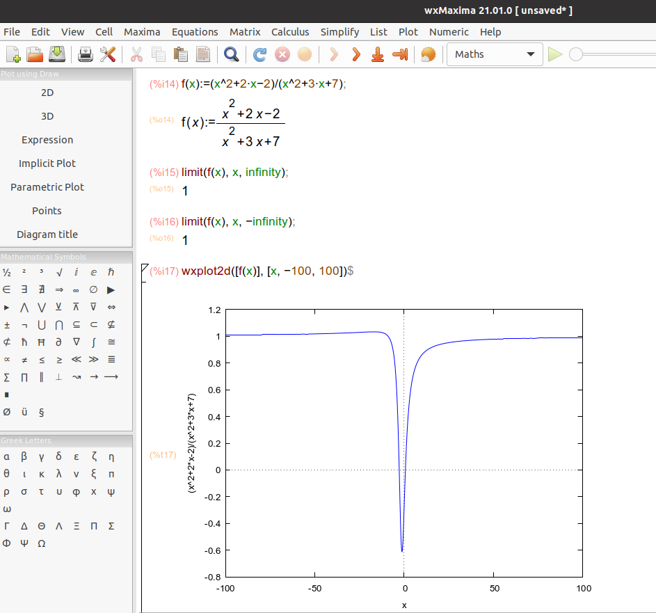

Continuous functions

A continuous function is a function that does not have any abrupt changes in value or discontinuities as the value of x changes. In other words, it is continuous at every point in its domain.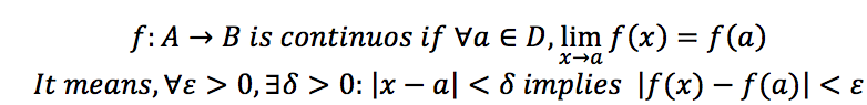

More intuitively, we can say that if we want to get all the f(x) values to stay in some small neighborhood or proximity around “f(a)”, we simply need to choose a small enough neighborhood for the x values around “a” or let’s put it in different terms, if we pick some x close enough to a, we ought to have f(x) close enough to “f(a)”.

Examples of continuous functions are polynomials (x, 2*x² − 7*x + 4), exponential function (e^x), sine function, cosine function, etc. ¹⁄_x is continuous whenever x is nonzero. However, ¹⁄_x is not defined at x=0, so it is discontinuous at x = 0.

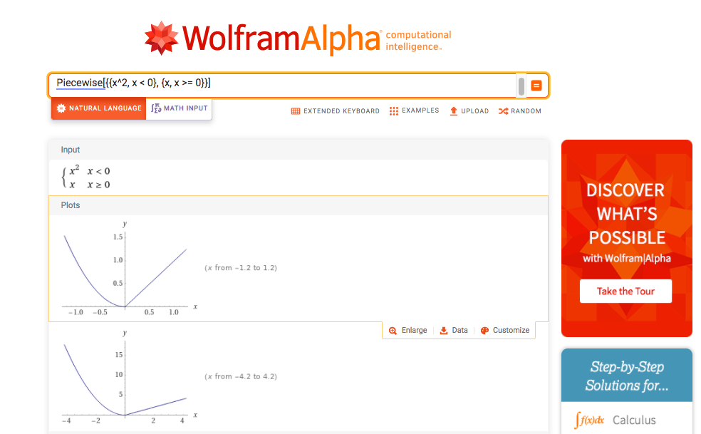
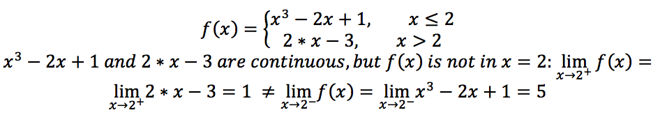
A piecewise function (a function defined by multiple sub-functions, where each sub-function applies to a different interval in the domain) is continuous if its constituent functions are continuous (x², x) on the corresponding intervals or subdomains, and there is no discontinuity at each endpoint of the subdomains (x = 0).

We are going to use WolframAlpha to demonstrate that the piecewise function f(x) is continuous: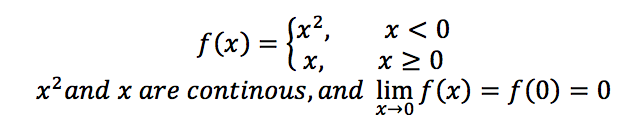

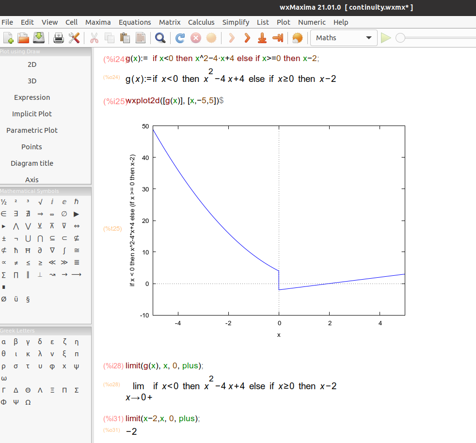
Let’s check in wxMaxima that the following piecewise function f(x) is continuous in all points except 0: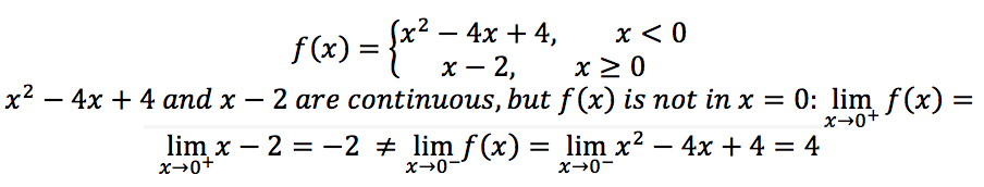

Finally, we will determine the continuity of a function in Python.

user@pc:~$ python
Python 3.8.10 (default, Jun  2 2021, 10:49:15) 
[GCC 10.3.0] on linux
Type "help", "copyright", "credits" or "license" for more information.
>>> from sympy import * # Import the SymPy library
>>> x = symbols('x')
>>> f = sp.Piecewise( (x**3-2*x+1, x<=2), (2*x-3, x > 2) ) 
# Represents a piecewise function. Each argument is a 2-tuple defining an expression and a condition.
>>> sp.limit(f, x, 2, '+') # SymPy can compute limits with the limit function. The syntax to compute is limit(f(x), x, a, dir). Limit's fourth argument, dir, specifies a direction.
1
>>> sp.limit(f, x, 2, '-')
5 # The function is not continuous at x = 2.
>>> from sympy.plotting import plot # The plotting module allows you to make 2-dimensional and 3-dimensional plots
>>> plot(f, (x, -5, 5), ylim=(-10,10), line_color='blue') # It plots the piecewise function. ylim denotes the y-axis limits and line_color specifies the color for the plot.

Derivative

The derivative of a function measures the sensitivity to change of the function value (output value) with respect to a change in its argument. The derivative of a function at a given point is the rate of change or slope of the tangent line to the function at that point.

Formally, y=f(x) is differentiable at a point “a” of its domain, if its domain contains an interval I containing a,

The command diff(expr, x) in Maxima returns the derivative or differential of expr with respect to x.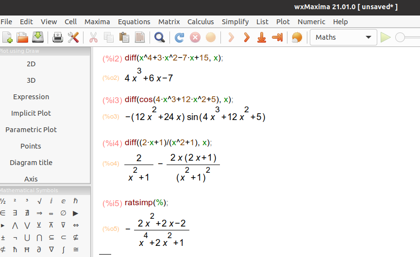

Remember some basic derivatives: f’(xⁿ) = n*xⁿ-1, (f(x)±g(x))’ = f’(x) ± g’(x) (they are needed for diff(x^4 +3*x^2- 7*x +15, x); cos’(x) = -sin(x), (f(g(x))’ = f’(g(x)) * g’(x) (diff(cos(4*x^3 +12*x^2 +5), x);)

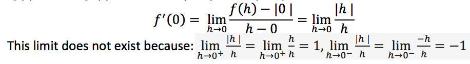
Let’s demonstrate that f(x)=|x| is continuous at x = 0, but is not differentiable at 0.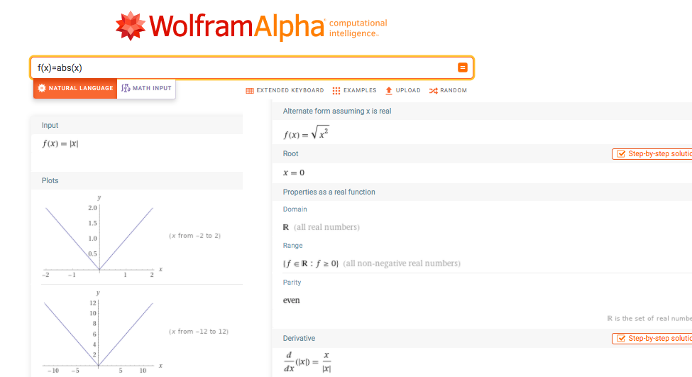

user@pc:~$ python # Let's do it with Python
Python 3.8.10 (default, Jun  2 2021, 10:49:15) 
[GCC 10.3.0] on linux
Type "help", "copyright", "credits" or "license" for more information.
>>> from sympy import * # Import the SymPy library
>>> x = symbols('x')
>>> init_printing(use_unicode=True) # To make it easier to read, we are going to enable pretty printing.
>>> diff(x**4+3*x**2-7*x+15, x) # To take derivatives, use the diff function.
   3          
4⋅x  + 6⋅x - 7
>>> diff(cos(4*x**3+12*x**2+5), x)
 ⎛    2      ⎞    ⎛  3       2    ⎞
-⎝12⋅x  + 24⋅x⎠⋅sin⎝4⋅x  + 12⋅x  + 5⎠
>>> diff((2*x+1)/(x**2+1), x)
  2⋅x⋅(2⋅x + 1)        2   
- ───────────── + ──────
            2        2    
    ⎛  2   ⎞       x  + 1
    ⎝x  + 1⎠            
>>> simplify(diff((2*x+1)/(x**2+1), x)) #  "One of the most useful features of SymPy is the ability to simplify mathematical expressions. SymPy has dozens of functions to perform various kinds of simplification and a general function called simplify() that attempts to apply all of these functions in an intelligent way to arrive at the simplest form of an expression," [Sympy's Manual](https://docs.sympy.org/latest/tutorial/simplification.html).
  ⎛   2        ⎞
2⋅⎝- x  - x + 1⎠
────────────────
   4     2      
 x  + 2⋅x  + 1  
>>>

The derivative of a function at a point is the slope of the tangent line at that point. It’s all abstract, so let’s show it graphically in Python.

user@pc:~$ python # Let's do it with Python
Python 3.8.10 (default, Jun  2 2021, 10:49:15) 
[GCC 10.3.0] on linux
Type "help", "copyright", "credits" or "license" for more information.
>>> from sympy import symbols, init_printing, diff, simplify # Import from the SymPy's library: symbols, init_printing, diff, and simplify.
>>> x = symbols('x')
>>> init_printing(use_unicode=True) # To make it easier to read, we are going to enable pretty printing.
>>> diff(x**2-3*x+4, x) # We use the diff function to derivative f(x) = x2 -3*x +4
2⋅x - 3
>>> diff(x**2-3*x+4, x).subs(x, 3) # The subs method replaces or substitutes all instances of a variable or expression with something else. 
3 # f'(3) = 3
>>> (x**2-3*x+4).subs(x, 3)
4 # f(3) = 4. The tangent line in x = 3 is: y = f'(3)(x - 3) + f(3) = 3(x -3) + 4 = 3*x -9 +4 = 3*x -5 
>>> from sympy.plotting import plot # The plotting module allows you to make 2-dimensional and 3-dimensional plots
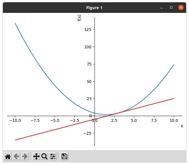
>>> p1 = plot(x**2-3*x+4, show=False) # It plots f(x). show=False, so it will not display the plot yet.
>>> p2 = plot(3*x-5, show=False, line_color='red') # It plots f'(x). show=False, so it will not display the plot yet. line_color='red' specifies the red color for the plot.
>>> p1.append(p2[0]) # To add the second plot’s first series object to the first, we use the append method.
>>> p1.show() # It displays the plot

L’Hôpital’s rule

It states that for two functions f and g which are differentiable on an interval I except possibly at a point “a” contained in I,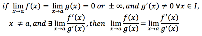

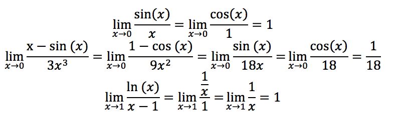
So, L’Hospital’s Rule is a great shortcut for doing some limits. It tells us that if we have a limit that produce an indeterminate form 0/0 (^sin(x)⁄_x, ^ln(x)⁄_x-1) or ∞/∞ all we need to do is differentiate the numerator and the denominator and then resolve the limit. However, sometimes, even repeated applications of the rule doesn’t help us to find the limit value.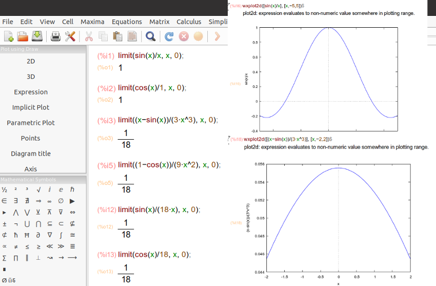

Series

A series is a description of the operation of adding infinitely many quantities, one after the other, to a given starting quantity. It can also be defined as the sum of a sequence, where a sequence is an ordered list of numbers (e.g., 1, 2, 3, 4,…. or 1, 2, 4, 8,…).

It is represented by an expression like a₁ + a₂ + a₃ + … or 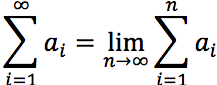When this limit exists, the sequence a₁ + a₂ + a₃ + … is summable or the series is convergent or summable and the limit is called the sum of the series. Otherwise, the series is said to be divergent.

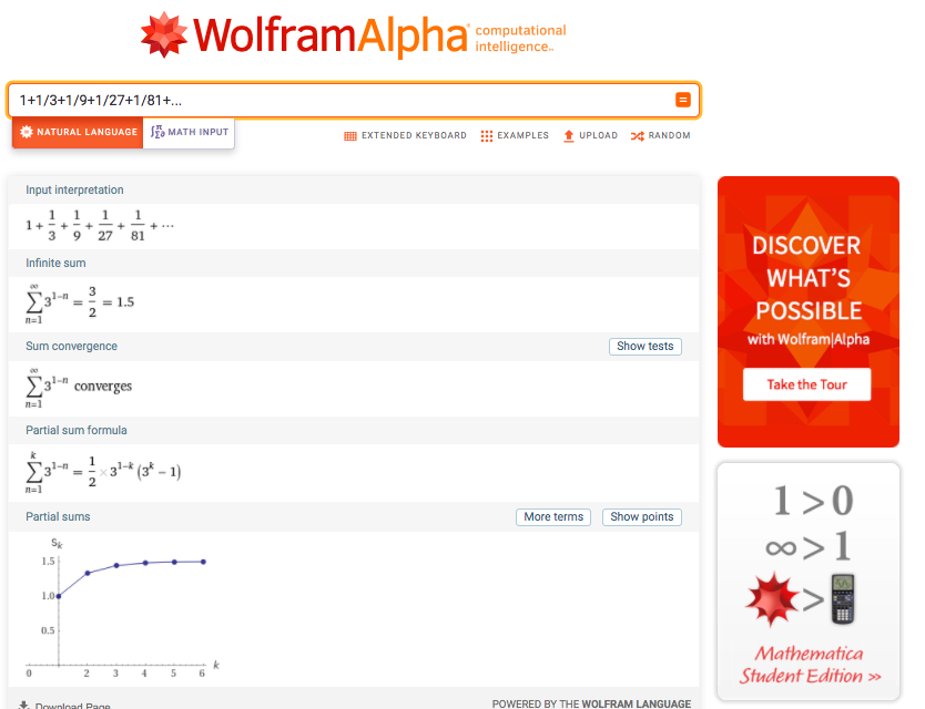
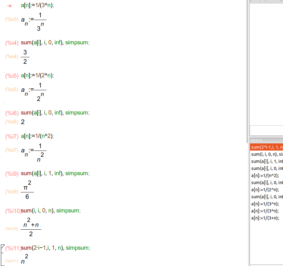
A geometric series is the sum of the terms of a geometric sequence (a sequence where each term after the first is found by multiplying the previous one by a fixed, non-zero number -it is usually called the common ratio r-: a, ar, ar², ar³…

The convergence of the geometric series depends on the value of the common ratio r. If |r|<1 (in the example above r=¹⁄₃), the series converges to the sum ^a⁄_1-r = ¹⁄_1-¹⁄3 = ¹⁄_²⁄3 = ³⁄₂ =1.5.

If r=1, all the terms are identical and the series is infinite. When r=-1, the terms take two values alternately (eg., 3, -3, 3, -3,…) and the sum of the terms oscillates between two values (3, 0, 3, 0, 3,…). Finally, if |r|>1, the sum of the terms gets larger and larger and the series is divergent. In conclusion, the series diverges if |r| ≥ 1.

Let’s work with wxMaxima. First, a![n]:=1/(3^n); defines a series. The basic command syntax is as follows: sum (a[i] -the expression to be summed-, i -the index-, 0 , inf -the upper and lower limits-), simpsum (it simplifies the result); Series in Maxima

a[n]:=1/(2^n); is a geometric series with r=¹⁄₂<1. It converges to the sum ^a⁄_1-r = ¹⁄_1-¹⁄2 = ¹⁄_¹⁄2 = 2. wxMaxima can compute other series, too: a[n]:=1/(n^2); it converges to ^π2⁄₆. We can find the sum of the first n terms of a series: sum(i, i, 0, n), simpsum; = ^{n2 + n}⁄₂ or sum(2*i-1,i, 1, n), simpsum; = n².

Let’s ask Wolfram Alpha about other series: sum(1/(n*(n+1)), n=1..infinity) (= 1), sum(1/(n^2), n=1..infinity) (= ^π2⁄₆), and sum((7*n^2+5*n-3)/(3*n^2-4*n+2), n=1..infinity). The last one diverges.

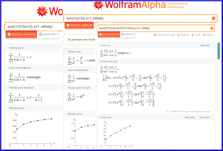
A simple test for the divergence of an infinite series is: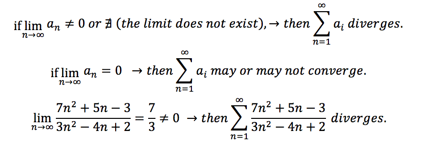

Integrals

Maxima can compute integrals of many functions. integrate (expr, x); attempts to symbolically compute the integral of expr with respect to x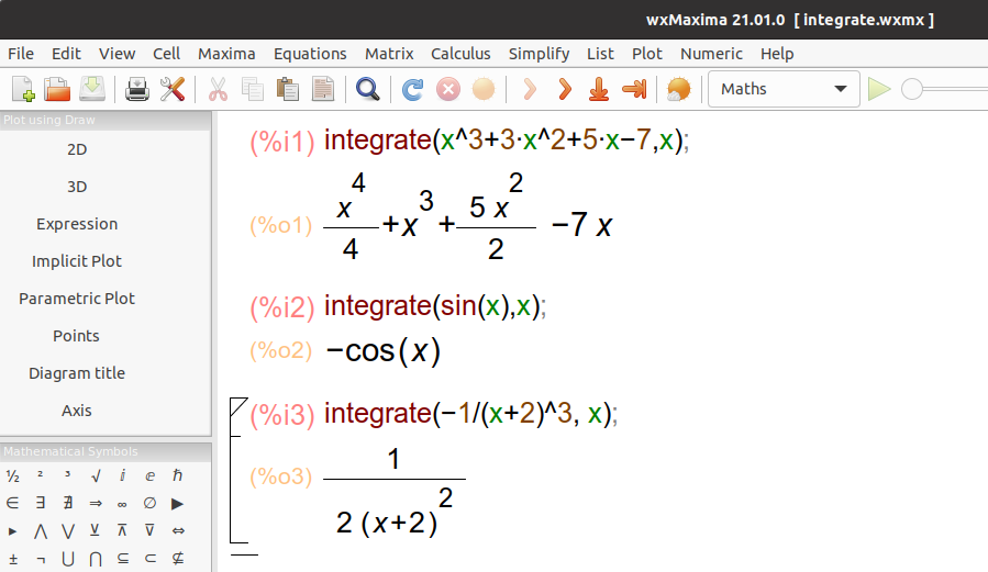

Wolfram|Alpha can compute indefinite and definite integrals, too, eg.: integrate x^2*(sin^3x) dx, integrate sin(x) dx, integrate x^3+3*x^2+5*x-7 dx, and integrate -1/(x+2)^3 dx.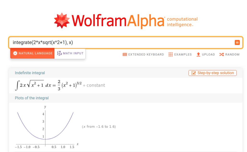

user@pc:~$ python # Let's do it with Python
Python 3.8.10 (default, Jun  2 2021, 10:49:15) 
[GCC 10.3.0] on linux
Type "help", "copyright", "credits" or "license" for more information.
>>> from sympy import *
>>> x = symbols('x')
>>> init_printing(use_unicode=True) # To make it easier to read, we are going to enable pretty printing.
>>> integrate(sin(x), x) # The integrals module in SymPy implements methods to calculate definite and indefinite integrals.
-cos(x)
>>> integrate(x**3+3*x**2+5*x-7, x)
 4           2      
x     3   5⋅x       
── + x  + ──── - 7⋅x
4          2        
>>> integrate(-1/(x+2)**3,x)
      1       
──────────────
   2          
2⋅x  + 8⋅x + 8
>>> integrate(2*x*sqrt(x**2+1),x)
         ________          ________
   2   ╱  2             ╱  2     
2⋅x ⋅╲╱  x  + 1      2⋅╲╱  x  + 1 
──────────────── + ─────────────  
       3                 3  

= ²⁄₃ (x²+1)(x²+1)^1⁄₂ = ²⁄₃ (x²+1)^3⁄₂

>>> integrate(x**3 +3*x**2 +5*x -7, (x, 1, 2)) 
# Sympy can calculate definite integrals: integrate(f, (x, a, b))
45/4
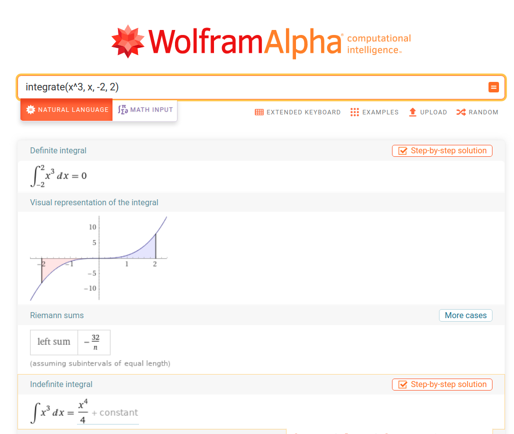
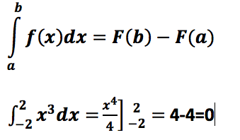
>>> integrate(x**3, (x, -2, 2))
0
>>> integrate(1/x, (x, 1, e))
1.00000000000000    

Going back to Maxima, integrate (expr, x) computes indefinite integrals, while integrate (expr, x, a, b) computes definite integrals, with limits of integration a and b.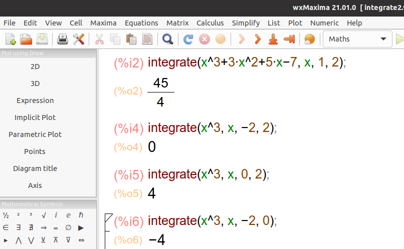

The solution to a definite integral gives you the signed area of the region that is bounded by the graph of a given function between two points in the real line. Conventionally, the area of the graph on or above the x-axis is defined as positive. The area of the graph below the x-axis is defined as negative.

Let f be a function defined on ![a, b] that admits an antiderivative F on [a, b] (f(x) = F’(x)). If f is integrable on [a, b] then, Definite integrals

Let’s see a few more examples.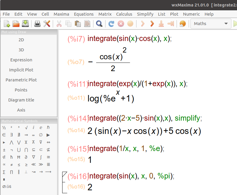

Taylor series

The Taylor series of a function f is a representation of this function as an infinite sum of terms that are calculated from the values of the function’s derivatives at a single point. Suppose f is a function that is infinitely differentiable at a point “a” in its domain. The Taylor series of f about a is the power series: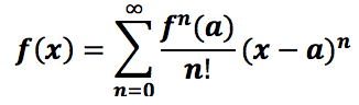

We start out with the Taylor series of the exponential function with base e at x=0: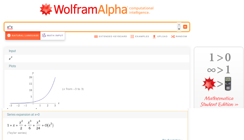

The derivative of the exponential function with base e is the function itself, (e^x)’=e^x.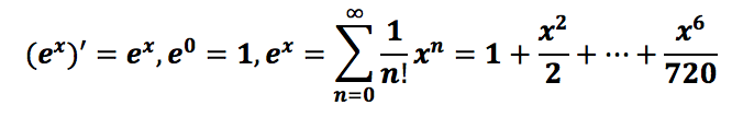

We can also specify the center point and the order of the expansion: series sin x at x=pi/2 to order 8, series ln (1-x) at x=0.

Maxima contains two functions (taylor and powerseries) for finding the series of differentiable functions. powerseries (expr, x, a) returns the general form of the power series expansion for expr in the variable x about the point a. taylor (expr, x, a, n) expands the expression expr in a truncated Taylor series in the variable x around the point a.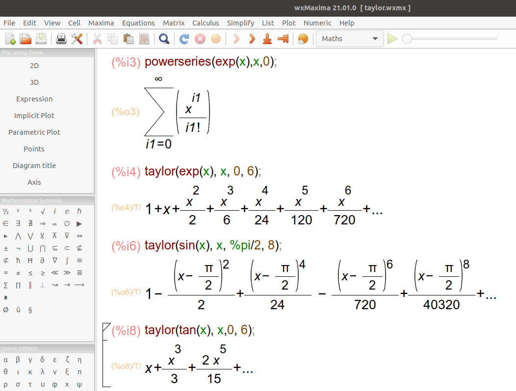

user@pc:~$ python # Let's do it with Python
Python 3.8.10 (default, Jun  2 2021, 10:49:15) 
[GCC 10.3.0] on linux
Type "help", "copyright", "credits" or "license" for more information.
>>> from sympy import * # Import the SymPy library
>>> x = symbols('x')
>>> init_printing(use_unicode=True) # To make it easier to read, we are going to enable pretty printing.
>>> series(cos(x),x) # series(expr, x, a, n) computes the series expansion of expr around point x = a. n is the number of terms up to which the series is to be expanded.
     2    4        
    x    x     ⎛ 6⎞
1 - ── + ── + O⎝x ⎠
    2    24        
>>> series(tan(x),x,0,6)
     3      5        
    x    2⋅x      ⎛ 6⎞
x + ── + ──── + O⎝x⎠
    3     15         
>>> series(ln(1-x),x)
       2    3    4    5        
      x    x    x    x      ⎛ 6⎞
-x - ── - ── - ── - ── + O⎝x ⎠
      2    3    4    5         
>>> series(exp(x),x)
         2    3    4     5        
        x    x    x     x      ⎛ 6⎞
1 + x + ── + ── + ── + ─── + O⎝x ⎠
        2    6    24   120        
>>> series(sin(x),x,pi/2,8)
           2         4         6                     
    ⎛    π⎞   ⎛    π⎞   ⎛    π⎞                      
    ⎜x - ─⎟   ⎜x - ─⎟   ⎜x - ─⎟   
    ⎝    2⎠   ⎝    2⎠   ⎝    2⎠   
1 - ──────── + ────── - ──────── + O(...)
        2         24         720