The Jacobian Matrix and Determinant

The real problem of humanity is the following: We have Paleolithic emotions, medieval institutions and godlike technology. And it is terrifically dangerous, and it is now approaching a point of crisis overall, Edward O. Wilson

Recall

So there are two notions of differentiability:

• Real differentiability of $F:\mathbb{R^{\mathnormal{2}}}\rightarrow \mathbb{R^{\mathnormal{2}}}$.
• Complex differentiability of $f:\mathbb{C}\rightarrow \mathbb{C}$.

They are related, but not the same. Complex differentiability is much more restrictive.

• Real differentiability: any linear map is allowed. For a function $F:\mathbb{R^{\mathnormal{2}}}\rightarrow \mathbb{R^{\mathnormal{2}}}$, real differentiability at a point $(x_0,y_0)$ means that there exists a real linear map $DF(x_0,y_0):\mathbb{R^{\mathnormal{2}}}\rightarrow \mathbb{R^{\mathnormal{2}}}$ (a $2\times 2$ matrix) such that
  $F(x_0+\Delta x,y_0+\Delta y)=F(x_0,y_0)+DF(x_0,y_0)\left( \begin{matrix}\Delta x\\ \Delta y\end{matrix}\right) +\mathrm{error},$ where the error is small compared to $\sqrt{(\Delta x)^2+(\Delta y)^2}.$
  So in the real sense, a function is differentiable if it can be locally approximated by a linear transformation (a matrix multiplication). This matrix can stretch, rotate, reflect, or skew space in any way.

• Complex differentiability: only complex multiplication is allowed. Now look at $f:\mathbb{C}\rightarrow \mathbb{C}$.
  Complex differentiability at $z_0$ means that there exists a complex number a such that $f(z_0+h)=f(z_0)+a\, h+\mathrm{error},$ where the error is small compared to |h| as $h\rightarrow 0$.
  In the real case, the linear approximation is any real-linear map $\mathbb{R^{\mathnormal{2}}}\rightarrow \mathbb{R^{\mathnormal{2}}}$. However, in the complex case, the linear approximation must be multiplication by a single complex number a, $a =re^{i\theta}$.
  Multiplication by a complex number $z$ results only in rotation by angle $\theta$ and uniform scaling by r = |a|. It does not allow for reflection or skewing.

Examples that show the difference

Example 1: $f(z) = z^2$. Write z = x + iy. Then, $z^ 2 = (x^2 - y^2) + i(2xy)$. So $u(x, y) = x^2 - y^2,\quad v(x, y) = 2xy.$

Compute partial derivatives: $u_x = 2x, u_y = -2y, $v_x = 2y, v_y = 2x$.

Check Cauchy–Riemann: $u_x = 2x, v_y = 2x,$ OK. $u_y = -2y,\ -v_x = -2y$, OK.

So f is complex differentiable everywhere. Its derivative is f’(z) = 2z. Geometrically, near each point $z_0$, it acts like multiplication by $2z_0$: rotation + scaling.

Example 2. The Conjugate Function. Let $f(z) = \bar{z} = x - iy$. This is the canonical counterexample showing that real differentiability does not imply complex differentiability.

1. Treating $\mathbb{C}$ as $\mathbb{R}^2$, we can write the function as a vector map $F: \mathbb{R}^2 \to \mathbb{R}^2$: $F(x, y) = \begin{pmatrix} x \\ -y \end{pmatrix}$
   This is a simple linear map. Since it is linear, it is infinitely differentiable (smooth) in the real sense. Its derivative is its Jacobian matrix, which is constant everywhere:
   $J_F = \begin{pmatrix} \frac{\partial u}{\partial x} & \frac{\partial u}{\partial y} \\ \frac{\partial v}{\partial x} & \frac{\partial v}{\partial y} \end{pmatrix} = \begin{pmatrix} 1 & 0 \\ 0 & -1 \end{pmatrix}$
2. For $f$ to be complex differentiable, its local linear approximation must be a complex linear map.
   A map $L: \mathbb{C} \to \mathbb{C}$ is complex linear if it is of the form $L(h) = \alpha \cdot h$ for some complex constant $\alpha = A + iB$.
   In matrix form, multiplication by $\alpha = A + iB$ corresponds to the specific matrix structure: $M_\alpha = \begin{pmatrix} A & -B \\ B & A \end{pmatrix}$
   

   This matrix represents a rotation (by $\arg \alpha$) and a scaling (by $|\alpha|$).

3. Now, compare the Real Jacobian of $\bar{z}$ with the required Complex Structure:
   $\text{Real Jacobian:} \begin{pmatrix} 1 & 0 \\ 0 & -1 \end{pmatrix} \quad \text{vs} \quad \text{Complex Form:} \begin{pmatrix} A & -B \\ B & A \end{pmatrix}$
   For these to match, we would need: Diagonals: $A = 1$ AND $A = -1$. Off-diagonals: $B = 0$ AND $-B = 0$.
   Condition (1) gives $1 = -1$, which is a contradiction.
   Therefore, the real derivative of $f(z) = \bar{z}$ exists, but it is not $\mathbb{C}$-linear.
4. The requirement that the Jacobian matches the “Complex Form” $\begin{pmatrix} A & -B \\ B & A \end{pmatrix}$ is exactly where the Cauchy-Riemann equations come from.
   For a general function $f(z) = u(x,y) + i v(x,y)$: $J_f = \begin{pmatrix} u_x & u_y \\ v_x & v_y \end{pmatrix} \overset{\text{must equal}}{\Longrightarrow} \begin{pmatrix} A & -B \\ B & A \end{pmatrix}$
   This implies: $u_x = v_y$ (The diagonals must match) and $u_y = -v_x$ (The off-diagonals must be opposite).
   Checking $f(z) = \bar{z}$: $u(x,y) = x \implies u_x = 1, \quad u_y = 0$; $v(x,y) = -y \implies v_x = 0, \quad v_y = -1$
   Check: $u_x = 1$ but $v_y = -1$.Result: $1 \neq -1$. The equations are not satisfied.

• Therefore, $f(z) = \bar{z}$ is not complex differentiable, even though it is smooth as a real function.

Geometric Interpretation:

• Complex Differentiable: Maps are Conformal (angle-preserving) and Orientation-preserving. They locally look like rotation + scaling.
• Complex Conjugate ($\bar{z}$): This is a Reflection across the x-axis. Reflections reverse orientation (like a mirror). Because it reverses orientation, it cannot be represented by rotation and scaling alone. Thus, it is not complex differentiable.

  In geometry and optics, reflections are classified as “opposite isometries” because they preserve the size and shape of a figure but reverse its orientation. This means that if you trace the vertices of a shape in a specific order (e.g., clockwise), the same vertices in the reflected image will appear in the opposite order (counterclockwise)

The Jacobian Matrix

Theorem. Let $F: U \subseteq \mathbb{R}^n \to \mathbb{R}^m$ be differentiable at a point $a \in U$, then, the derivative $DF_a: \mathbb{R}^n \to \mathbb{R}^m$ is a linear map whose matrix with respect to the standard bases of $\mathbb{R}^n$ and $\mathbb{R}^m$ is the Jacobian matrix $J_F(a) = \begin{pmatrix} \frac{\partial F_1}{\partial x_1}(a) & \frac{\partial F_1}{\partial x_2}(a) & \cdots & \frac{\partial F_1}{\partial x_n}(a) \\ \frac{\partial F_2}{\partial x_1}(a) & \frac{\partial F_2}{\partial x_2}(a) & \cdots & \frac{\partial F_2}{\partial x_n}(a) \\ \vdots & \vdots & \ddots & \vdots \\ \frac{\partial F_m}{\partial x_1}(a) & \frac{\partial F_m}{\partial x_2}(a) & \cdots & \frac{\partial F_m}{\partial x_n}(a) \end{pmatrix} = \begin{pmatrix} | & | & & | \\[4pt] \frac{\partial F}{\partial x_1}(a) & \frac{\partial F}{\partial x_2}(a) & \cdots & \frac{\partial F}{\partial x_n}(a) \\[4pt] | & | & & | \end{pmatrix}$ (the Jacobian matrix $J_F(a)$ is formed by all partial derivatives). In other words, for every h = $(h_1, h_2, \cdots, h_n)^T \in \mathbb{R}^n$, $\boxed{DF_a(h) = J_F(a) \cdot h}$

That is, the derivative (a linear map) is represented by the Jacobian matrix and the matrix for $DF_a$ has columns equal to the partial derivatives. ∎

Proof.

1. Differentiability definition:
   There exists a linear map L: ℝⁿ → ℝᵐ such that:
   $\lim_{h \to 0} \frac{\|F(a + h) - F(a) - L(h)\|}{\|h\|} = 0$
2. Matrix representation. Choose the standard basis $\{e_1, \cdots, e_n\}$ for $\mathbb{R}^n$ and $\{e_1', \cdots, e_m'\}$ for $\mathbb{R}^m$. The matrix of L with respect to these bases is the m × n matrix whose j-th column is $L(e_j)$ (written in $\mathbb{R}^m$ coordinates).
3. Compute $L(e_j)$ using the definition. Set $h = te_j$ with $t \ne 0$. As $t \to 0$: $\frac{F(a + te_j) - F(a)}{t} -L(e_j) = \frac{1}{t}[F(a + te_j) - F(a)-L(te_j)]$
   $\frac{1}{t}[F(a + te_j) - F(a)-L(te_j)] [\text{ Because }\frac{\|F(a + h) - F(a) - L(h)\|}{\|h\|} \to 0 \text{ Substitute } h = te_j] \to 0.$
   Hence, $L(e_j) = \lim_{t \to 0}\frac{F(a + te_j) - F(a)}{t} = \frac{\partial F}{\partial x_j}(a)$
4. Interpretation of the partial derivative: $\frac{\partial F}{\partial x_j}(a)$ is a vector in $\mathbb{R}^m$; its i-th component is $\frac{\partial F_i}{\partial x_j}(a)$. Therefore, the j-th column of the matrix of L is precisely: $\biggr(\begin{smallmatrix}\frac{\partial F_1}{\partial x_j}(a) \\\ \frac{\partial F_2}{\partial x_j}(a) \\\ . \\\ . \\\ . \frac{\partial F_m}{\partial x_j}(a)\end{smallmatrix}\biggl)$
5. The matrix of L is exactly the Jacobian matrix $J_F(a).$

Important Remarks

1. The theorem states that if F is differentiable at a, then all partial derivatives exist and the derivative’s matrix is the Jacobian. The converse is false – a function may have all partial derivatives at a yet fail to be differentiable.
   Theorem. Sufficient Condition for Differentiability. If all partial derivatives $\frac{\partial F_i}{\partial x_j}$ exist in a neighborhood of a and are continuous at a, then F is differentiable at a.
   This condition is often written as “$F \in C^1$” or “F is continuously differentiable.”
2. Linear Approximation Formula. If F is differentiable at a, then for small h: $F(a + h) \approx F(a) + J_F(a) \cdot h$. This is the first‑order Taylor expansion in several variables.
   In components, if $h = (h_1, h_2, \ldots, h_n)$: $F_i(a + h) \approx F_i(a) + \sum_{j=1}^{n} \frac{\partial F_i}{\partial x_j}(a) \cdot h_j$
3. Theorem (Chain Rule). Let F: U ⊆ ℝⁿ → ℝᵐ and G: V ⊆ ℝᵐ → ℝᵖ where F(U) ⊆ V. If F is differentiable at a and G is differentiable at F(a), then G ∘ F is differentiable at a with: $D(G \circ F)_a = DG_{F(a)} \circ DF_a$
   In matrix form: $J_{G \circ F}(a) = J_G(F(a)) \cdot J_F(a)$
   This is a direct consequence of the representation theorem above and the chain rule for derivatives.

Illustrative Examples

• Let $F(x,y) = (x^2 - y^2, 2xy)$.

Compute partial derivatives: $\frac{\partial F}{\partial x} = (2x, 2y), \frac{\partial F}{\partial y} = (-2y, 2x)$.

Jacobian at (x, y): $J_F(x,y) = \begin{pmatrix} 2x & -2y \\ 2y & 2x \end{pmatrix}.$

For any $\mathbf{h} = (h, k), DF_{(x,y)}(h,k) = J_F(x,y)\begin{pmatrix}h\\k\end{pmatrix} = \begin{pmatrix} 2x h - 2y k \\ 2y h + 2x k \end{pmatrix}.$

This matches the complex derivative view, $f(z) = z^2$, $f'(z)=2z$.

• Counterexample. Consider $f(x, y) = \begin{cases} \frac{xy}{x^2 + y^2} & (x, y) \neq (0, 0) \\ 0 & (x, y) = (0, 0) \end{cases}$

Partial derivatives measure rates of change along coordinate axes only (e.g., x-axis or y-axis). Differentiability requires the function to behave linearly in ALL directions simultaneously (it requires the function to be well-approximated by a linear map in every direction near the point).

Formally, the limit $\lim_{h \to 0} \frac{\|F(a + h) - F(a) - L(h)\|}{\|h\|} = 0$ must hold. For f to be differentiable at (0, 0), this limit must exist regardless of the path $(h, k) \to (0, 0).$

Partial derivatives at origin exist: $\frac{\partial f}{\partial x}(0, 0) = \lim_{t \to 0} \frac{f(t, 0) - f(0, 0)}{t} = \lim_{t \to 0} \frac{0 - 0}{t} = 0$ and $\frac{\partial f}{\partial y}(0, 0) = \lim_{t \to 0} \frac{f(0, t) - f(0, 0)}{t} = \lim_{t \to 0} \frac{0 - 0}{t} = 0$ because the function is identically zero along the axes.

But f is NOT differentiable at origin:

If f were differentiable at (0,0), then $Df_{(0,0)}(h, k) = \frac{\partial f}{\partial x}(0, 0)\cdot h + \frac{\partial f}{\partial x}(0, 0)\cdot k = 0\cdot h + 0 \cdot k = 0$ (the zero map), so: $\lim_{(h,k) \to (0,0)} \frac{|f(h, k) - f(0, 0) - 0|}{\sqrt{h^2 + k^2}} = \lim_{(h,k) \to (0,0)} \frac{|hk|}{(h^2 + k^2)^{3/2}}$

However, along the path h = k = t: $\frac{|t^2|}{(2t^2)^{3/2}} = \frac{t^2}{2\sqrt{2}|t|^3} = \frac{1}{2\sqrt{2}|t|} \to \infty$ as $t \to 0$.

This path-dependent divergence proves the limit does not exist, violating the definition of differentiability.

The graph of f near (0, 0) resembles a “saddle” with sharp ridges along the lines y = x and y = −x. While the function is flat along the axes (where partial derivatives exist), it rises steeply along other paths (e.g., y = x), preventing a linear approximation from capturing its behavior.

• Let F: ℝ² → ℝ² with F(s,t) = (s², st) and G: ℝ² → ℝ with G(u,v) = u + v².

Recall. Chain Rule, $J_{G \circ F}(a) = J_G(F(a)) \cdot J_F(a)$

Jacobians: $J_F(s,t) = \begin{pmatrix} 2s & 0 \\ t & s \end{pmatrix}, J_G(u,v) = \begin{pmatrix} 1 & 2v \end{pmatrix}$

At point (s,t) = (2, 3): F(2, 3) = (4, 6), $J_F(2,3) = \begin{pmatrix} 4 & 0 \\ 3 & 2 \end{pmatrix}, \quad J_G(4, 6) = \begin{pmatrix} 1 & 12 \end{pmatrix}$

Chain rule (matrix multiplication): $J_{G \circ F}(2, 3) = J_G(4,6) \cdot J_F(2,3) = \begin{pmatrix} 1 & 12 \end{pmatrix} \begin{pmatrix} 4 & 0 \\ 3 & 2 \end{pmatrix} = \begin{pmatrix} 40 & 24 \end{pmatrix}$

Verification: $(G \circ F)(s,t) = s^2 + (st)^2 = s^2 + s^2t^2$

$\frac{\partial(G \circ F)}{\partial s} = 2s + 2st^2 = 2⋅2+2⋅2⋅9=4+36=40 \checkmark$

$\frac{\partial(G \circ F)}{\partial t} = 2s^2 t = 2⋅4⋅3=24 \checkmark$

Special Cases and Terminology

When F: ℝⁿ → ℝ is a scalar-valued function, the Jacobian is a 1 × n row vector: $J_f(a) = \begin{pmatrix} \frac{\partial f}{\partial x_1}(a) & \frac{\partial f}{\partial x_2}(a) & \cdots & \frac{\partial f}{\partial x_n}(a) \end{pmatrix}$

The gradient is the same information, but arranged as an n x 1 column vector: $\nabla f(a) = \begin{pmatrix} \frac{\partial f}{\partial x_1}(a) \\[6pt] \frac{\partial f}{\partial x_2}(a) \\[6pt] \vdots \\[6pt] \frac{\partial f}{\partial x_n}(a) \end{pmatrix}$ Important remarks:

• $J_f = (\nabla f)^T$.
• The Jacobian is the linear map that best approximates f near a.
• The gradient is the vector that points in the direction of steepest ascent.
• Linear approximation: $f(a + h) \approx f(a) + \nabla f(a) \cdot h$

  This is the multivariable version of the tangent line. The dot product expresses how the function changes in the direction of h.

When γ: ℝ → ℝᵐ is a curve (n = 1), the Jacobian is an m × 1 column vector: $J_\gamma(t) = \begin{pmatrix} \gamma_1'(t) \\ \gamma_2'(t) \\ \vdots \\ \gamma_m'(t) \end{pmatrix} = \gamma'(t)$. This is the velocity vector of the curve at parameter t (direction of motion, speed).

The Jacobian as a Scaling Factor

When F: ℝⁿ → ℝⁿ (n = m), the Jacobian $J_F$ is a square n × n matrix. In this case, the determinant det($J_F$) is well-defined.

For a smooth function $F: \mathbb{R}^n \to \mathbb{R}^n$, the Jacobian matrix $J_F$ represents the best linear approximation of the function near a specific point.

If you zoom in very close to a point $a$, the function $F$ behaves like a linear transformation (matrix multiplication).

• A linear transformation $T(x) = Ax$ maps a unit cube to a parallelepiped.

  The Jacobian determinant measures the local scaling of volume (or area) induced by a transformation. To see this, consider a small rectangle in the (u, v)-plane with sides du and dv. Under the transformation F, this rectangle is mapped to a parallelogram in the (x, y)-plane. The area of this parallelogram is approximately: $\text{Area} \approx |\vec{r}_u \times \vec{r}_v| du dv$ where $\vec{r}_u$ and $\vec{r}_v$ are the tangent vectors obtained by differentiating the transformation with respect to u and v, respectively. The magnitude of their cross product is precisely the absolute value of the Jacobian determinant. Thus, the Jacobian determinant quantifies how much an infinitesimal area (or volume) is stretched or compressed by the transformation at each point.

• The volume of that resulting parallelepiped is exactly $|\det(A)|$.
• Therefore, for a general non-linear function $F$, the absolute value of the Jacobian determinant, $|\det(J_F)|$, tells us the local volume expansion (or contraction) factor.
• If $|\det(J_F)| = 2$, the function is locally stretching space, doubling volumes. If $|\det(J_F)| = 0.5$, the function is locally compressing space, halving volumes. If $|\det(J_F)| = 0$, the mapping squashes dimension (flattening a 2D area onto a 1D line or point).

Let’s apply this to the transformation from polar coordinates $(r, \theta)$ to Cartesian coordinates $(x, y)$.

The Map: $F(r, \theta) = \begin{pmatrix} r \cos \theta \\ r \sin \theta \end{pmatrix} = \begin{pmatrix} x \\ y \end{pmatrix}$

To find the Jacobian Matrix $J_F$, we take the partial derivatives of $x$ and $y$ with respect to $r$ and $\theta$: $J_F = \frac{\partial(x, y)}{\partial(r, \theta)} = \begin{pmatrix} \frac{\partial x}{\partial r} & \frac{\partial x}{\partial \theta} \\ \frac{\partial y}{\partial r} & \frac{\partial y}{\partial \theta} \end{pmatrix} = \begin{pmatrix} \cos\theta & -r\sin\theta \\ \sin\theta & r\cos\theta \end{pmatrix}$

Now we calculate the determinant: $\det(J_F) = (\cos\theta)(r\cos\theta) - (-r\sin\theta)(\sin\theta)= r\cos^2\theta + r\sin^2\theta = r(\cos^2\theta + \sin^2\theta) = r$

Imagine a tiny rectangle in the “Input Space” (the $r\theta$-plane) defined by a small change in radius $\Delta r$ and a small change in angle $\Delta \theta$.

Input Area: $\Delta A_{input} \approx \Delta r \cdot \Delta \theta$.

Now map this rectangle to the “Output Space” (the $xy$-plane). It becomes a curved polar sector.

• Radial Direction: The side corresponding to $\Delta r$ stretches directly outward. Its length is simply $\Delta r$.
• Tangential Direction: The side corresponding to the angle change $\Delta \theta$ is an arc. The length of an arc is not just the angle; it is the radius times the angle. Arc Length $\approx r \cdot \Delta \theta$.
• The resulting shape is approximately a rectangle with sides $\Delta r$ and $r \Delta \theta$. $\Delta A_{output} \approx (\text{radial length}) \times (\text{arc length})$. Hence, $\Delta A_{output} \approx (\Delta r) \times (r \Delta \theta) = r (\Delta r \Delta \theta)$

  This visually confirms what the determinant told us: the area scales by a factor of $r$. The further out you go (larger $r$), the “wider” the angular sectors become, covering more Cartesian area for the same change in angle.

This geometric scaling is the reason behind the Change of Variables formula in multiple integrals. If we want to integrate a function $f(x, y)$ over a region $D$, and we switch to polar coordinates, we must replace the area element $dx dy$ with the scaled area element:

$$\iint_D f(x, y) dxdy = \iint_{D'} f(r \cos\theta, r \sin\theta) \underbrace{|\det(J_F)|}_{\text{Scaling Factor}} dr d\theta = \iint_{D'} f(r, \theta) r dr d\theta$$

Without the correcting factor $|J| = r$, we would be treating the wide outer rings of the polar grid as having the same area as the tiny inner rings, which would give an incorrect result.

Take the surface $z = 9 -x^2 -y^2$ and let’s say that we want to calculate the volume under the surface but above the xy-plane.

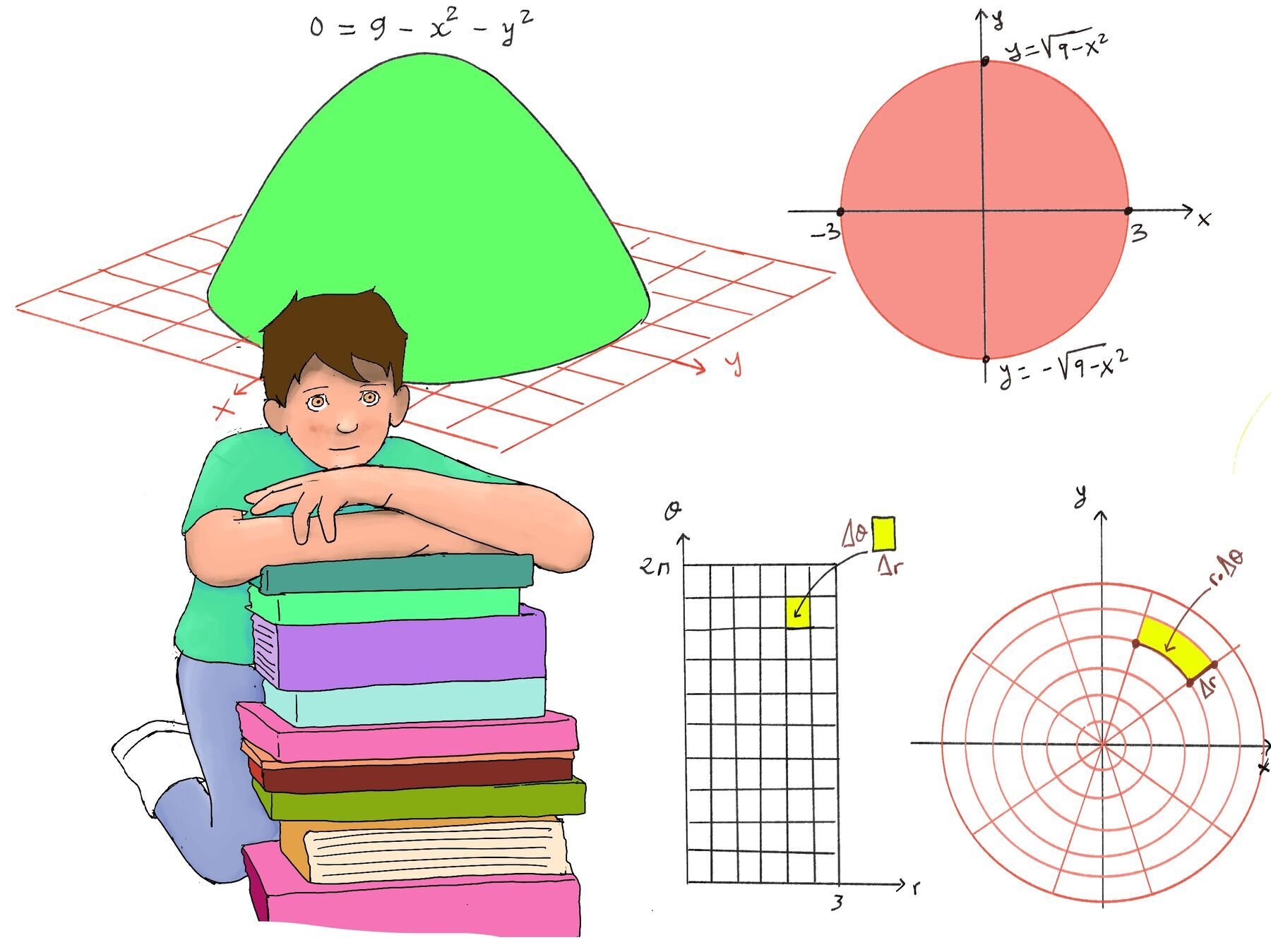
$\int_{-3}^3 \int_{-\sqrt{9-x^2}}^{\sqrt{9-x^2}} (9 -x^2-y^2)dydx = \int_{0}^{2\pi} \int_{0}^{3} -r^2 |det(J(r, \theta))| drd\theta = \int_{0}^{2\pi} \int_{0}^{3} -r^3drd\theta$

Compute the Inner Integral: $\int_{0}^{3} -r^3 dr = \int_{0}^{3} -r^3 dr = -\left[ \frac{1}{4} r^4 \right]_03 = -\frac{1}{4} (3^4 - 0) = -\frac{1}{4} (81) = -20.25$

Compute the Outer Integral: V = $\int_0^{2\pi} (-20.25) d\theta = -20.25 \cdot (2\pi) = -40.5\pi$

The negative sign indicates that the surface lies below the xy-plane. If we are interested in the magnitude of the volume (i.e., the unsigned measure), we can report $40.5\pi$ as the volume.