Curves in the Complex Plane: Definitions and Properties

Irony is wasted on the stupid, Oscar Wilde

Introduction

The complex plane is a two-dimensional coordinate system where:

• The horizontal axis (real axis) represents the real part of a complex number.
• The vertical axis (imaginary axis) represents the imaginary part. Any complex number $z = a + bi $ (where $a, b \in \mathbb{R} $) is plotted as the point $(a, b)$.

In complex analysis, curves provide the paths along which we integrate complex functions. A curve $\gamma$ in the complex plane is essentially a continuous, one-dimensional path trace by a function of a real parameter t.

Definition. A curve $\gamma$ in the complex plane is a continuous function $\gamma: [a, b] \to \mathbb{C}$ defined on a closed interval $[a, b] \subset \mathbb{R}$. The parameter $t\in[a,b]$ represents position along the curve, and as $t$ increases from a to b, $\gamma(t)$ moves through the complex plane, tracing out the path.

The image (or trace) of $\gamma$ is the set of points traced or visited: $\gamma^* = \{\gamma(t) : a \leq t \leq b\}$. If $\gamma^* \subseteq S$ for some region $S \subseteq \mathbb{C}$, $S \subseteq \mathbb{C}$, we say $\gamma$ is contained or lies in $S$. The starting or initial point of $\gamma$ is $\gamma(a)$ and the ending, terminal or final point is $\gamma(b)$.

Since $\gamma(t)$ is a complex number for each $t$, we can decompose it into real and imaginary parts: $\gamma(t) = x(t) + iy(t),$ where $x, y : [a, b] \to \mathbb{R}$ are real-valued functions. The continuity of $\gamma$ is equivalent to the continuity of both $x(t)$ and $y(t)$.

Orientation: The direction in which t increases defines the curve’s orientation (e.g., clockwise vs. counterclockwise) — the “arrow” indicating which way the path is traversed. Traversing from $t = a$ to $t = b$ follows the positive direction of the curve. Traversing from t = a to t = b follows the positive direction of the curve. Reversing the direction corresponds to traversing from b back to a.

Opposite Curve: Given a curve $\gamma: [a,b] \to \mathbb{C}$, the opposite or reversed curve $-\gamma$ is defined on the same interval $[a,b]$ by $(-\gamma)(t) = \gamma(a + b - t)$ for $t \in [a,b]$. This means $-\gamma$ traces the same set of points as $\gamma$ but in the opposite or reverse direction (starting where $\gamma$ ended, and ending where $\gamma$ began).

Examples of Common Curves

Straight Lines

A straight line between two points $z_0$ and $z_1$ is parametrized as: $\boxed{\gamma(t) = z_0 + t(z_1 - z_0)}, t \in [0, 1]$.
At $t = 0$: $\gamma(0) = z_0$. At $t = 1$: $\gamma(1) = z_1$. For $t \in (0, 1)$, $\gamma(t)$ is a convex combination of $z_0$ and $z_1$, producing points on the line segment between them.
Example: From $z_0 = 1 + 2i$ to $z_1 = 3 + 4i$: $\gamma(t) = 1 + 2i + t(2 + 2i) = (1 + 2t) + i(2 + 2t)$.

Circles and Ellipses

• A circle of radius $R > 0$ centered at $z_0 \in \mathbb{C}$, traversed counterclockwise is parametrized as: $\boxed{\gamma(t) = z_0 + Re^{it}}, \qquad t \in [0, 2\pi].$
• Unit Circle: $\gamma(t) = e^{it} = \cos t + i \sin t, t \in [0, 2\pi]$. This traces a circle of radius 1 ($|z| = 1$) counterclockwise centered at the origin.
  For a clockwise traversal, reverse the sign of $t$: $\gamma(t) = e^{-it}$, $t \in [0, 2\pi]$.
• Ellipse. An ellipse centered at the origin with semi-axes $a > 0$ (horizontal) and $b > 0$ (vertical): $\boxed{\gamma(t) = a \cos t + i b \sin t}, a, b > 0, \qquad t \in [0, 2\pi]$. If we write z = x + i·y, then: x(t) = acos(t), y(t) = bsin(t). Solve for cosine and sine, $\cos t=\frac{x}{a}, \sin t=\frac{y}{b}$ which is valid because a, b > 0 so we can divide by them. The fundamental identity $\cos^2(t)+\sin^2(t)=1$ holds for all t. Substitute the expressions above, and we get: $\frac{x^2}{a^2} + \frac{y^2}{b^2} = 1$. That’s the standard Cartesian equation of an ellipse centered at the origin with semi-axes a (along x) and b (along y).
  For a = 2, b = 1, it forms a horizontally stretched ellipse.
  When $a = b = R$, this reduces to a circle of radius $R$.

  When a > b, the ellipse is stretched horizontally. The curve is traced counterclockwise as t increases from 0 to $2\pi.$

Parabolas and Higher-Degree Curves

• Parabola: $\gamma(t) = t + it^2, t \in [-2, 2]$. This traces a parabola in the complex plane (real part linear, imaginary part quadratic). If z = x + i y, then comparing real and imaginary parts: $x(t) = t, y(t) = t^2.$ From x(t) = t, we immediately get: t = x. Substitute into y(t) = t²: y = x². Cartesian equation. The curve satisfies $y = x^2, x \in [-2, 2].$ That’s the standard equation of a parabola opening upward with vertex at the origin, axis of symmetry along the y-axis; domain restricted to [-2, 2] because t is in that range; Range: $y \in [0, 4]$. It traces the familiar U-shaped parabola in the (x, y) plane.

• Logarithmic Spirals: $\gamma(t) = e^{kt} e^{i\theta t} =[\text{Using Euler’s formula}] e^{kt} (\cos \theta t + i \sin \theta t), k, \theta \in \mathbb{R}$. Real and imaginary parts. If z = x + i y, then: $x(t) = e^{kt}\cos(\theta t), y(t) = e^{kt} \sin(\theta t)$.
  In polar form $z = r e^{i\varphi}$: Radius: $r(t) = e^{kt}$. This grows (if $k > 0$) or shrinks (if $k < 0$) exponentially with t. Angle: $\varphi(t) = \theta t$ (rotating at constant angular speed). So the curve is a logarithmic spiral, meaning that the distance from the origin changes exponentially while the angle changes at a constant rate.

Example: For k = 1, $\theta = 1, x(t) = e^{t} \cos(t), y(t) = e^{t} \sin(t)$. Radius: $r(t) = e^{t}$ — grows rapidly as t increases. Angle: $\varphi(t) = t$ — rotates (changes) at a constant speed. As $t \to \infty$, the spiral winds outward, getting farther from the origin each turn. As $t \to -\infty$, $r(t) \to 0$, causing the spiral to wind inward toward the origin.
Special cases: $k = 0$: a circle of radius $1$ (no radial growth).
$\theta = 0$: a ray from the origin along the positive real axis (no rotation).

Curvature

Curvature measures how sharply a curve bends at a given point.. Formally, for a smooth curve in the plane or space parametrized by $\mathbf{r}(t) = (x(t), y(t))$ with $\mathbf{r}'(t) \neq \mathbf{0}$:, the curvature $\kappa$ at a point is defined as: $\kappa = \left\lVert \frac{d\mathbf{T}}{ds} \right\rVert$ where:

• $\mathbf{T}$ is the unit tangent vector to the curve,
• s is the arc-length parameter,
• $\frac{d\mathbf{T}}{ds}$ is the rate of change of the tangent direction per unit length along the curve.

If a curve is given by a smooth vector function $\mathbf{r}(t) = \big(x(t), y(t)\big) \ \text{or in 3D: } (x(t), y(t), z(t))$ and $\mathbf{r}'(t) \neq \mathbf{0}$, then the unit tangent vector is: $\mathbf{T}(t) = \frac{\mathbf{r}'(t)}{\|\mathbf{r}'(t)\|}$

• $\mathbf{r}'(t)$ is the velocity vector (derivative of position with respect to t).
• $\|\mathbf{r}'(t)\|$ is its magnitude (speed).
• Dividing by the magnitude makes it a unit vector (length 1).

Imagine driving along the curve: curvature tells you how quickly you have to turn the steering wheel at that point.
A straight line r(t) = a + tb, where b is a constant vector. The tangent vector $\mathbf{T}$ is constant (since r’(t) = b), therefore $\frac{\mathbf{dT}}{ds} = 0$, it has curvature 0 (no turning require).
A circle of radius R, r(t) = (Rcos(t), Rsin(t)) has constant curvature $\kappa = \frac{1}{R}$ — smaller circles bend more sharply, so they have higher curvature.

$\mathbf{T}(t)$ points along the curve in the direction of motion. It ignores how fast you’re moving — only the direction matters.

Closed and Simple Curves

Definition. A curve $\gamma: [a, b] \to \mathbb{C}$ is closed if its starting point coincides with its endpoint, i.e., γ(a) = γ(b). In other words, a closed curve forms a loop with no gap between its beginning and end, e.g.,

• The unit circle parametrized by $\gamma(t) = e^{2\pi i t}, t \in [0, 1]$ is closed since $\gamma(0) = \gamma(1) = 1$ (both the start and end point are $1$ on the complex plane).
• Ellipse: $\gamma(t) = 2\cos(t) + i\sin(t), t \in [0, 2\pi]$ is a closed ellipse with horizontal semi-axis of length 2 and vertical semi-axis of length 1 (both the start and end point are 2 on the complex plane, $\gamma(0) = \gamma(2\pi) = 2$).
• Figure-8 Curve: $\gamma(t) = \cos(t) + i \cos(2t), t \in [0, 2\pi]$ is closed but self-intersecting.

  Writing it in real–imaginary coordinates: $x(t) = \cos(t), y(t) = \cos(2t)$. At $t = \frac{\pi}{2} \text{ and } \frac{3\pi}{2}$, we get the same point $(0, -1)$, so the path crosses itself.

Definition. A curve $\gamma: [a, b] \to \mathbb{C}$ is simple if γ(t₁) = γ(t₂) if it does not intersect itself (no self-crossings), except possibly at the endpoints when the curve is closed. Formally, if $\gamma(t_1) = \gamma(t_2) \Rightarrow \begin{cases} t_1 = t_2, & \text{for a non-closed (open) curve}, \\ \{t_1, t_2\} = \{a, b\}, & \text{for a closed curve}. \end{cases}$.

The only repetition allowed is $\gamma(a) = \gamma(b)$. In words, the image of $\gamma$ has no repeated points, except that a closed simple curve (also called a loop and a Jordan curve) may have its start and end points coincide.

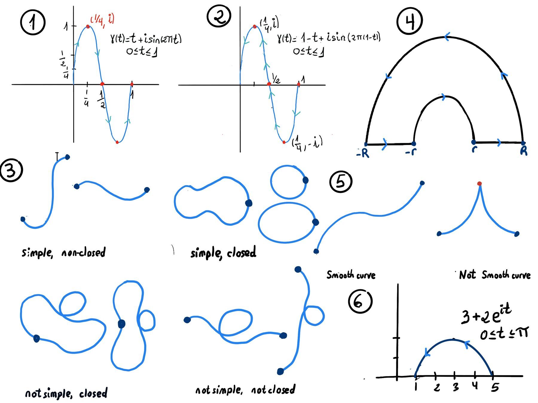Figure 3. Simple/not simple, closed/non-closed curves.

Examples:

• Open Simple Curve: The line segment from 0 to 1 + i ( (0,0) to (1,1) ): $\gamma(t) = t(1+i), t \in [0, 1]$ is simple because it never intersects itself. It is open because the endpoints are distinct: γ(0) = 0 and γ(1) = 1+i. Length: $1+i = \sqrt{2}$. Curvature: Zero everywhere (straight line).
• Closed Simple Curve: The unit circle parametrized by $\gamma(t) = e^{2\pi i t}, t \in [0, 1]$ is simple. Using Euler’s formula $e^{i\theta} = \cos(\theta) + i(\sin(\theta))$, we can write: $\gamma(t) = \cos(2\pi t) + i \sin(2\pi t)$, the curve is the unit circle in the complex plane, centered at the origin. At t = 0: $\gamma(0) = 1 + 0i$. At t = 1: $\gamma(1) = e^{2\pi i} = 1 + 0i$ the curve meets itself again. The curve’s orientation is counterclockwise as t increases from 0 to 1.
• Example of Non-Simple Curve: $z(t) = e^{it}$ for t from 0 to 4π traces the unit circle twice, making it non-simple due to self-intersection at t = 2π.
• Figure-eight (self-intersecting). $\gamma(t) = \cos t + i\cos 2t$, $t \in [0, 2\pi]$ is not simple.

Joining Curves (Concatenation)

Often we build complicated paths by joining simpler curve segments end-to-end. If one curve ends at the point where another begins, we can concatenate them.

Definition (Join of Two Curves). Let $\gamma_1 : [a, b] \to \mathbb{C}, \text{ and } \gamma_2 : [c, d] \to \mathbb{C}$ be two curves such that the endpoint of the first curve $\gamma_1$ matches the starting point of the second $\gamma_2$: $\gamma_1(b) = \gamma_2(c)$. The join (or concatenation) of $\gamma_1$ and $\gamma_2$ is the new curve $\gamma_1 * \gamma_2$ obtained by traversing $\gamma_1$ first and then $\gamma_2$. Formally, we can define $(\gamma_1 \ast \gamma_2) : [a,\, b + (d - c)] \to \mathbb{C}$ defined by $(\gamma_1+\gamma_2)(t) = \begin{cases} \gamma_1(t), & a \le t \le b, \\ \gamma_2\big(t - b + c\big), & b < t \le b + (d - c). \end{cases}$.

Here we have reparameterized the second curve $\gamma_2$ to immediately follow $\gamma_1$ in parameter time. The new curve $\gamma_1 * \gamma_2$ starts at $\gamma_1(a)$ and ends at $\gamma_2(d)$, passing through $\gamma_1(b)=\gamma_2(c)$ at the “joining” point.

This idea extends naturally to any finite sequence of curves: if $\gamma_2$ starts where $\gamma_1$ ends, $\gamma_3$ starts where $\gamma_2$ ends, and so on, then we can join them one after another.

Join of n Curves. Given a chain of curves $\gamma_1 : [a_1, b_1] \to \mathbb{C}, \gamma_2 : [a_2, b_2] \to \mathbb{C}, \dots, \gamma_n : [a_n, b_n] \to \mathbb{C}$ with $\gamma_{i-1}(b_{i-1}) = \gamma_i(a_i), \text{for } 2 \le i \le n,$ their concatenation $\gamma_1 * \gamma_2 * \cdots * \gamma_n$ is the curve obtained by concatenating them in order, reparametrizing each so that the next starts where the previous ends.

Examples

• Two Straight Segments (open path). Let $\gamma_1(t) = t, t \in [0, 1]$. This parametrizes a straight line from 0 to 1 in $\mathbb{C}$ (along the real axis). $\gamma_2(s) = 1 + it, t \in [0, 1]$. This parametrizes a straight line from 1 to 1 + i, a vertical line segment of length 1 in the imaginary direction. Here $\gamma_1(1) = 1 = \gamma_2(0)$, so they can be joined: $(\gamma_1 \ast \gamma_2)(t) = \begin{cases} t, & 0 \le t \le 1, \\ 1 + i(t - 1), & 1 < t \le 2. \end{cases}$.

The overall path forms an “L-shape”; it goes right along the real axis from 0 to 1, then up parallel to the imaginary axis (1 + i).

• Semicircle Followed by Line (Closed Loop). Let $\gamma_1(t) = e^{i\pi t}, t \in [0, 1]$ which traces the upper semicircle from 1 (when t = 0) to -1 (when t = 1) along the unit circle (radius 1, counterclockwise), and let $\gamma_2(s) = -1 + s, s \in [0, 2]$ which is a line segment from -1 to 1 along the real axis (passing through 0). Since $\gamma_1(1) = -1 = \gamma_2(0)$, these two curves can be concatenated. The joined curve $\gamma_1 * \gamma_2$ forms a closed loop: it goes from 1 to -1 along the upper half of the unit circle, then returns from -1 back to 1 along the real line, so this path is closed. It traces a “D”-shaped curve composed of a semicircular arc and a line segment.

$(\gamma_1 \ast \gamma_2)(t) = \begin{cases} e^{i\pi t}, & t\in[0,1],\\[4pt] -1 + (t-1), & t\in[1,3]. \end{cases}$.

• Three-Segment Polygonal Path (Three Sides of a Triangle). Let’s join multiple line segments in sequence. Let $\gamma_1(t) = t, t \in [0, 1]$ from 0 to 1 along the real axis; $\gamma_2(t) = 1 + it, t \in [0,1]$: from 1 to 1 + i vertical segment upward, and $\gamma_3(t) = (1-t) + i(1-t), t \in [0, 1]$: moves diagonally downward-left from 1 + i back to 0. Each $\gamma_i$ is a straight line on $\mathbb{C}$. If we concatenate $\gamma_1 * \gamma_2 * \gamma_3$, the resulting path goes from 0 to 1, from 1 to 1 + i, then returns from 1 + i back to 0. This traces three sides of a triangle in the complex plane with vertices 0, 1, and 1 + i. The result is a simple closed contour.

$(\gamma_1 \ast \gamma_2 \ast \gamma_3)(t) = \begin{cases} t, & t\in[0,1],\\[4pt] 1+i(t-1), & t\in[1,2],\\[4pt] (3-t)+i(3-t), & t\in[2,3]. \end{cases}$.

When concatenating $\gamma_1, \gamma_2$ and $\gamma_3$​, the total path is parameterized over $t \in [0, 3]$. The third segment corresponds to $t \in [2, 3]$, so we reparameterize $\gamma_3$​ as follows: Let s = t − 2, where $s \in [0, 1]$ when $t \in [2, 3]$. Substitute s into $\gamma_3(s) = (1-s) + i(1-s)$. Replace s with t−2, $(\gamma_1 \ast \gamma_2 \ast \gamma_3)(t) = (1−(t−2))+i(1−(t−2))=(3−t)+i(3−t), t\in [2,3]$.

• Opposite Paths Traversing the Same Points. Consider the curve γ₁(t) = t + isin(2πt), 0 ≤ t ≤ 1. This starts at γ₁(0) = 0 and ends at γ₁(1) = 1. For example, γ₁(0) = 0 + isin(0) = 0, γ₁(1/4) = 1/4 + isin(π/2) = 1/4 + i, γ₁(1/2) = 1/2 + isin(π) = 1/2, γ₁(3/4) = 3/4 - i, γ₁(1) = 1 + isin(2π) = 1.

Now consider another curve γ₂(t) = 1 - t + isin(2π(1 - t)), 0 ≤ t ≤ 1. This starts at γ₂(0) = 1 and ends at γ₂(1) = 0. For example, γ₂(0) = 1 + isin(0) = 1, γ₂(1/4) = 3/4 + isin(2π·3/4) = 3/4 + isin(3π/2) = 3/4 - i, γ₂(3/4) = 1/4 + i, γ₂(1) = 0. Both curves trace the same set of points in the complex plane: a real-axis segment from 0 to 1 with a sinusoidal oscillation in the imaginary part. However, the direction of traversal is opposite: γ₁ goes from 0 to 1, γ₂ goes from 1 to 0. γ₂ is exactly the opposite curve of γ₁ (Figures 1 and 2).

We can find an explicit reparameterization function $\phi: [0,1] \to [0,1]$ such that $\gamma_2(t) = \gamma_1(\phi(t))$. If we guess $\phi(t) = 1 - t$, then $\gamma_1(1 - t) = (1-t) + i\sin(2\pi(1-t))$, which is precisely $\gamma_2(t)$. Thus $\phi(t)=1-t$ reverses the path.

$(\gamma_1 \ast \gamma_2)(t) = \begin{cases} t+i\sin(2\pi t), & t\in[0,1],\\[6pt] 2-t+i\sin\big(2\pi(2-t)\big), & t\in[1,2]. \end{cases}$.

Note: $\gamma_2(t-1)=1-(t-1)+i\sin\!\big(2\pi(1-(t-1))\big)=2-t+i\sin\big(2\pi(2-t)\big)$

• A Closed Contour Around an Annulus. Let r, R ∈ $\mathbb{R}, 0 < r < R$ be two real radii, we want to define the curve illustrated in the figure 4, a closed piecewise path that loops around the annular region between the circle of radius r and the circle of radius R.

1. Outer radial segment: γ₁(t) = r(1 - t) + Rt, 0 ≤ t ≤ 1. This is a straight line from r to R along the positive real axis.
2. Outer circular arc: γ₂(t) = Re^it, 0 ≤ t ≤ π. This is the upper semicircle of radius R from R (t = 0) to -R (t = π), traversed counterclockwise along the outer circle.
3. Inner radial segment: γ₃(t) = -R(1-t) -rt, 0 ≤ t ≤ 1. This is a straight line from -R to -r along the negative real axis.
4. Inner circular arc: γ₄(t) = re^-it, -π ≤ t ≤ 0. This is a lower semicircle of radius r, running from -r back to r (traversed clockwise).

$(\gamma_1 \ast \gamma_2 \ast \gamma_3 \ast \gamma_4)(t) = \begin{cases} r(1 - t) + Rt, & 0 \le t \le 1, \\ Re^{i(t-1)}, & 1 \le t \le \pi + 1, \\ -R(\pi + 2 -t) -r(t - (\pi +1)), & \pi + 1 \le t \le \pi + 2, \\ -re^{i(t-(\pi+2))}, & \pi+2 \le t \le 2\pi + 2 \end{cases}$.

This concatenation forms a closed contour that encloses the annular region between the two concentric circles of radii r and R, with overall counterclockwise orientation (Figure 4).

Smooth Curves and Contours

Not all continuous curves are “nice” enough for calculus purposes; we often restrict to curves that are differentiable and without sudden changes in direction.

Definition. A curve $\gamma: [a, b] \to \mathbb{C}$ is smooth if it is continuously differentiable on $(a,b)$ and its derivative never vanishes on $[a,b]$.

What “Smooth” Really Mean (Figure 5):

1. The derivative $\gamma'(t)$ exists for all t and is continuous on the interval [a, b]. A smooth curve’s direction changes only gradually, it doesn’t have any sharp corners or cusps (a point on a curve where the direction changes abruptly).
2. The derivative is never zero: $\gamma'(t) \ne 0 \text{ for all t } \in [a, b]$. Non-vanishing derivative guarantees that the curve is one-to-one (locally injective) and has a well-defined tangent direction at every point — no “stopping” or “looping back” (it does not retrace itself locally) on itself in an infinitesimal neighborhood. There are no cusps or instant reversals of direction because that would require the velocity to drop to zero before changing direction.

Together, these conditions imply that the curve is regular and differentiable, with a smooth trajectory through the complex plane. It is one you could trace with a pen in a single motion, without lifting it or hitting a snag. It flows continuously and nicely through the plane, and at every point, you can clearly see or say this is the direction it’s heading.

Why does non-zero derivative imply local injectivity? Imagine walking along a path. If your velocity (derivative) never becomes zero, you’re always moving forward — never standing still or turning back. That guarantees you won’t step on the same spot twice (you won’t hit the same point twice) in a small stretch (interval). In short, a continuously nonzero velocity ensures the curve doesn’t intersect itself in a small neighborhood, and it has a clear direction at every point.

Definition. A path or contour in the complex plane is a curve that is made up of a finite sequence (finitely many) of smooth pieces or curves joined end-to-end. In other words, a contour is a piecewise smooth curve. Formally, $\Gamma$ is a contour if $\Gamma = \gamma_1 * \gamma_2 * \cdots * \gamma_n$ for some finite collection of smooth curves $\gamma_1, \dots, \gamma_n$. Key points about contours:

• Each segment $\gamma_i$ is smooth: it has a continuous, non-zero derivative.
• The overall path $\Gamma$ is piecewise smooth, meaning it may have corners or bends at the junctions between segments, but it has no breaks or discontinuities. There are only finitely many points (the join points) where the derivative might not be defined or might change direction abruptly.
• If the contour is closed (start and end coincide), we often call it a closed contour. A simple closed contour is one that does not cross itself (a loop with no self-intersections, like a circle).
• In complex integration theory, contours are the paths along which we integrate complex functions. A piecewise smooth path is sufficient for defining $\int_\Gamma f(z)dz$.
• We often name contours by their geometric shape or the region they bound. For example: a circle contour of radius R ($\gamma(t) = Re^{it}, 0 \le t \le 2\pi$) is a closed contour (smooth and simple) oriented counterclockwise; a semicircle contour (e.g., the upper half of a circle, $\gamma(t) = Re^{it}, 0 \le t \le \pi$); a polygonal contour (e.g., a triangle or rectangle formed by joining three or four line segments). These are piecewise linear (each segment smooth) and the whole loop is piecewise smooth (corners at the vertices); an annulus contour, a path that goes around an annular region (sometimes used to integrate around a hole between two circles).

Computational Implementation

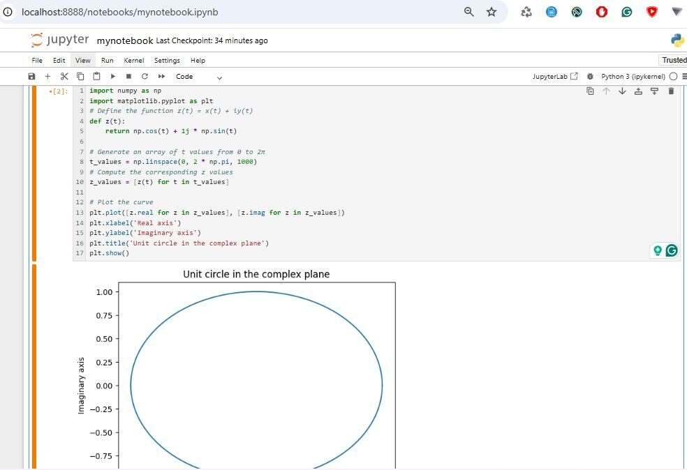
The computational implementation of curves in the complex plane involves using numerical methods to approximate the curve and its derivatives. One common approach is to use the numpy library in Python to perform numerical computations and the matplotlib library to visualize the curve.

Here is an example code snippet that demonstrates how to plot a curve in the complex plane:

import numpy as np
import matplotlib.pyplot as plt

# Define the function z(t) = x(t) + iy(t)
# This function represents a point on the unit circle in the complex plane,
# where x(t) = cos(t) and y(t) = sin(t).
def z(t):
    return np.cos(t) + 1j * np.sin(t)  # Return complex number z as x + iy
    # j is the imaginary unit (mathematicians often use i, but in Python it’s j).
    # It can be rewritten using Euler's formula directly as return np.exp(1j * t)
    # np.cos(t) is the x-coordinate, np.sin(t) is the y-coordinate.
    # If t = 0: cos(0) + i·sin(0) = 1 + 0i, point at (1, 0) on the circle.
    # If t = π/2: cos(π/2) + isin(π/2) = 0 + i, point at (0, 1) on the circle.

# Generate an array of t values from 0 to 2π
# This will create 1000 evenly spaced values in the range [0, 2π],
# which are used to parameterize the unit circle.
t_values = np.linspace(0, 2 * np.pi, 1000)

# Compute the corresponding z values for each t
# Using a list comprehension, we apply the function z(t) to each t value
# to get the corresponding complex numbers on the unit circle.
z_values = [z(t) for t in t_values]

# Plot the curve
# Extract or unpack the real and imaginary parts of the complex numbers for plotting.
plt.plot([z.real for z in z_values], [z.imag for z in z_values])
plt.xlabel('Real axis')  # Label for the x-axis
plt.ylabel('Imaginary axis')  # Label for the y-axis
plt.title('Unit Circle in the Complex Plane')  # Plot title
plt.axis('equal')  # Set equal scaling for both axes
plt.grid()  # Add a grid for better visualization
plt.show()  # Display the plot

Curves in the complex plane are fundamental tools across mathematics, physics, and engineering. Their study enhances understanding of function behavior, physical phenomena, and engineering systems. Whether through integration paths or modeling wavefunctions, these curves provide essential insights into various fields.