Parametric Curves and Polar Coordinates

“Mr. Smith, could you explain to us what recursion is all about?” The professor in Introduction to Programming asked an apathetic student. “I don’t know the question, but sex, money, or both is definitely the answer, and God, justice, our values, and love are just the excuses,” I replied. “You shall not pass,” the teacher was far from amused, Apocalypse, Anawim, #justtothepoint.

Parametric Curves

Parametric curves are mathematical descriptions of curves using one or more independent variables, called parameters.

Instead of expressing a direct relationship between $x$ and $y$ (like $y = x^2$), parametric equations define both $x$ and $y$ (and potentially $z$ in 3D space) as individual functions of a shared parameter. This parameter is often denoted by $t$ (representing time), $u$, or $\theta$ (representing an angle).

In two dimensions, a parametric curve is defined by a pair of equations: $x = f(t)$ and $y = g(t)$

Example 1: The Circle

A classic example of a parametric curve is a circle with radius $a$, defined by: $x = a\cos(t)$ and $y = a\sin(t)$

We can verify this forms a circle by substituting these into the standard Cartesian equation for a circle, $x^2 + y^2 = a^2$:

Since $\cos^2(t) + \sin^2(t) = 1$, this simplifies perfectly to $a^2$ (Figure 2.f.).

If we track the trajectory as $t$ increases:

• At $t = 0$, the position is $(x, y) = (a\cos(0), a\sin(0)) = (a, 0)$.
• At $t = \frac{\pi}{2}$, the position is $(x, y) = (a\cos(\frac{\pi}{2}), a\sin(\frac{\pi}{2})) = (0, a)$.

This means the curve is drawn counter-clockwise starting from the positive x-axis.

Arc Length of the Circle

1. To calculate the arc length (the distance traveled along the curve), we use the differential formula $ds = \sqrt{(\frac{dx}{dt})^2 + (\frac{dy}{dt})^2}dt$.
2. $\frac{dx}{dt} = -a\sin(t)$, $\frac{dy}{dt} = a\cos(t)$
3. $ds = \sqrt{(-a\sin(t))^2 + (a\cos(t))^2}dt = \sqrt{a^2(\sin^2(t) + \cos^2(t))}dt = \sqrt{a^2}dt = a dt$

The speed (rate of change $\frac{ds}{dt}$) is exactly $a$. Integrating this from $0$ to $2\pi$ gives the circumference: $2\pi a$.

Example 2: The Ellipse

Consider a slightly different set of equations: $x = 2\sin(t)$ and $y = \cos(t)$

Notice what happens if we square and manipulate them: $\frac{x^2}{4} + y^2 = \sin^2(t) + \cos^2(t) = 1$ (Figure 1.a.).

 .

Recall. The equation $\frac{x^2}{a^2} + \frac{y^2}{b^2} = 1$ is the standard form of an ellipse centered at the origin $(0, 0)$.

Let’s track this trajectory:

• At $t = 0$, $(x, y) = (2\sin(0), \cos(0)) = (0, 1)$.
• At $t = \frac{\pi}{2}$, $(x, y) = (2\sin(\frac{\pi}{2}), \cos(\frac{\pi}{2})) = (2, 0)$.

Unlike the circle, this parametrization traces the ellipse clockwise, starting from the positive y-axis.

Arc Length and Surface Area

The speed along this ellipse is $\frac{ds}{dt} = \sqrt{(2\cos(t))^2 + (-\sin(t))^2} = \sqrt{4\cos^2(t) + \sin^2(t)}$.

To find the total arc length, we set up the integral: $\text{Arc Length} = \int_{0}^{2\pi} \sqrt{4\cos^2(t) + \sin^2(t)}dt$

However, unlike the circle, this is an “elliptic integral” and cannot be solved using basic elementary functions; it requires numerical approximation.

If we revolve the right half of this ellipse ($t$ from $0$ to $\pi$) around the y-axis (Figure 1.b.), we generate a 3D ellipsoid. The surface area of revolution is given by $S = \int 2\pi x \, ds$: $S = \int_{0}^{\pi} 2\pi(2\sin(t))\sqrt{4\cos^2(t) + \sin^2(t)}dt$

Polar Coordinates

While Cartesian coordinates $(x, y)$ map points on a rectangular grid, polar coordinates map points based on a circular grid originating from a central pole.

Polar coordinates are an alternative way of specifying the position of a point in a 2D plane using two quantities: the radial distance ($r$) and the angular coordinate ($\theta$) where:

• $r$ represents the straight-line distance from the origin (the pole) to the point.
• $\theta$ is the angle measured counter-clockwise from the positive x-axis (the polar axis). We typically assume $0 \le \theta < 2\pi$.

Converting Between Systems

You can seamlessly translate between Cartesian $(x, y)$ and Polar $(r, \theta)$ using right-triangle trigonometry:

• $x = r\cos(\theta)$ and $y = r\sin(\theta)$
• $r = \sqrt{x^2 + y^2}$ and $\theta = \arctan(\frac{y}{x})$

Example: Convert the Cartesian point $(1, -1)$ to polar.

1. $r = \sqrt{1^2 + (-1)^2} = \sqrt{2}$
2. $\theta = \arctan(\frac{-1}{1}) = -\frac{\pi}{4}$ (which is geometrically in the fourth quadrant, or $315^\circ$).

The polar coordinate is $(\sqrt{2}, -\frac{\pi}{4})$.

Graphing in Polar Coordinates

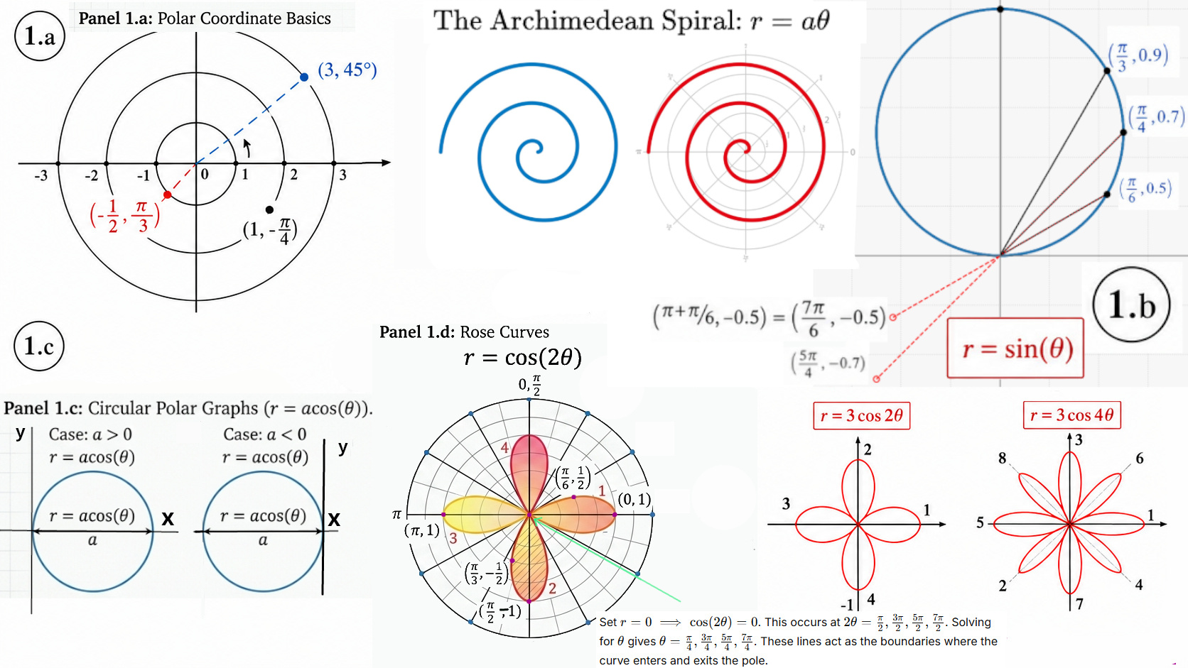
Plotting points is straightforward: for $(3, 45^\circ)$, you face the $45^\circ$ angle and walk exactly 3 units outward from the center. But what happens if the radius is negative?

Rule of Negative Radii: When graphing a polar coordinate with a negative radius, you face the given angle, but move backward from the pole in the exact opposite direction.

For example, consider the point $(-\frac{1}{2}, \frac{\pi}{3})$. The negative sign dictates direction, not distance (distance is always absolute). You face $\frac{\pi}{3}$ ($60^\circ$), but step backward $\frac{1}{2}$ units. This lands you in the exact same spot as if you faced the opposite angle and walked forward: $(\frac{1}{2}, \frac{\pi}{3} + \pi) = (\frac{1}{2}, \frac{4\pi}{3})$ (Figure 1.a).

If we convert this to Cartesian:

• $x = -\frac{1}{2}\cos(\frac{\pi}{3}) = -\frac{1}{4}$
• $y = -\frac{1}{2}\sin(\frac{\pi}{3}) = -\frac{\sqrt{3}}{4}$

Exploring Polar Curves

Polar functions usually take the form $r = f(\theta)$. By changing the function, we can create incredibly complex and beautiful shapes.

Famous Polar Shapes

The Archimedean Spiral

Defined by $r = a\theta$, this curve represents a spiral with a constant rate of increase in radial distance as the angle increases. Because the distance between turnings is constant, it looks like a coiled rope.

Polar Rose Curves

Equations of the form $r = a\cos(k\theta)$ or $r = a\sin(k\theta)$ generate “leafed roses.” The constant $a$ determines the length of each petal, while the integer $k$ dictates the number of petals:

• If $k$ is an odd integer, the rose will have exactly $k$ petals, e.g., $r = 3\cos(3\theta)$ yields a 3-petal rose.
• If $k$ is an even integer, the rose will have $2k$ petals, e.g., $r = 3\cos(2\theta)$ yields a 4-petal rose.

For example, $r = 3\cos(2\theta)$ produces a 4-petal rose. The tip of each petal reaches exactly $3$ units from the center. The first petal of a cosine rose will always align with the positive x-axis ($\theta = 0$).

The Impact of a Negative Radius

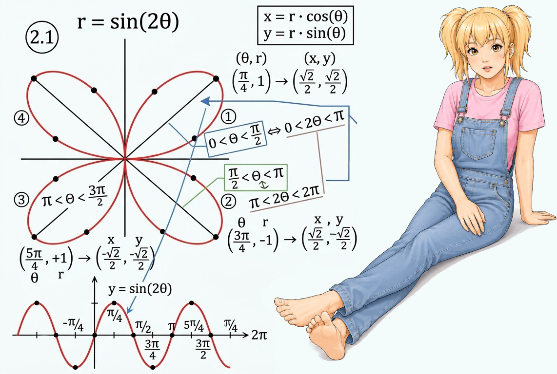
Consider the four-leaved rose $r = \sin(2\theta)$ (Figure 2.1). If we test a few points to trace it:

• At $\theta = 0$, $r = 0$.
• At $\theta = \frac{\pi}{4}$, $r = 1$ (the tip of the first petal in Quadrant I).
• At $\theta = \frac{\pi}{2}$, $r = 0$.
• When $\theta$ enters the second quadrant ($\frac{\pi}{2} < \theta < \pi$), $2\theta$ falls between $\pi$ and $2\pi$, causing $\sin(2\theta)$ to become negative. A negative radius means the coordinate is plotted in the opposite direction (rotated 180° or $\pi$ radians through the origin). Therefore, even though the angle $\theta$ is sweeping through the second quadrant, the curve is actually being drawn in the fourth quadrant.

Circles in Polar Coordinates

Circles can be expressed elegantly in polar coordinates depending on their placement relative to the origin.

Circles Centered on an Axis

If you trace the polar curve $r = \sin(\theta)$ (Figure 1.b.):

1. Look along the positive x-axis ($\theta = 0$): $r = \sin(0) = 0$.
2. Turn slowly to the left ($\theta > 0$): The radius increases ($\sin(\frac{\pi}{6}) = 0.5$, $\sin(\frac{\pi}{4}) \approx 0.7$, etc.).
3. The radius tops out at $1$ when $\theta = \frac{\pi}{2}$ (along the positive y-axis).
4. As you continue to turn, it comes back to the origin when $\theta = \pi$.
5. As you turn toward the negative y-direction ($\pi < \theta \leq 2\pi$), the radius becomes negative, which completely retraces the original circle in the upper half-plane.

Similarly, $r = a\cos(\theta)$ represents a circle shifted along the x-axis. It sits to the right if $a > 0$ and to the left if $a < 0$, with a total diameter of $a$ (Figure 1.c.).

Deriving the Off-Center Circle Equation

To express the equation of a circle centered at $(a, 0)$ with radius $a$ (Figure 1.d.), we start with its standard Cartesian equation, $(x - a)^2 + y^2 = a^2 \implies x^2 - 2ax + a^2 + y^2 = a^2 \implies (x^2 + y^2) - 2ax = 0$

Then, we convert to polar coordinates, using the substitutions $r^2 = x^2 + y^2$ and $x = r\cos(\theta)$: $r^2 - 2a(r\cos(\theta)) = 0$

Factoring out $r$ yields the solutions $r = 0$ (the origin) and the complete circle equation: $\boxed{r = 2a\cos(\theta)}$

Area in Polar Coordinates

To find the area enclosed by a polar curve, we use circular sectors instead of the rectangular strips used in Cartesian integration.

The area of a full circle is $\pi r^2$. A sector represents a fraction of that circle based on its angle $\Delta\theta$. The percentage of the total area is $\frac{\Delta\theta}{2\pi}$. Therefore, the area of a small sector is: $\boxed{\Delta A = \left(\frac{\Delta\theta}{2\pi}\right) \pi r^2 = \frac{1}{2}r^2 \Delta\theta}$ (Figure 1.a.)

At an infinitesimal scale, this becomes $dA = \frac{1}{2}r^2 d\theta$.

To find the total area swept between two angles, we integrate: $\boxed{\text{Area} = \int_{\theta_1}^{\theta_2} \frac{1}{2}r^2 \, d\theta}$ (Figure 1.b).

Area of the Off-Center Circle

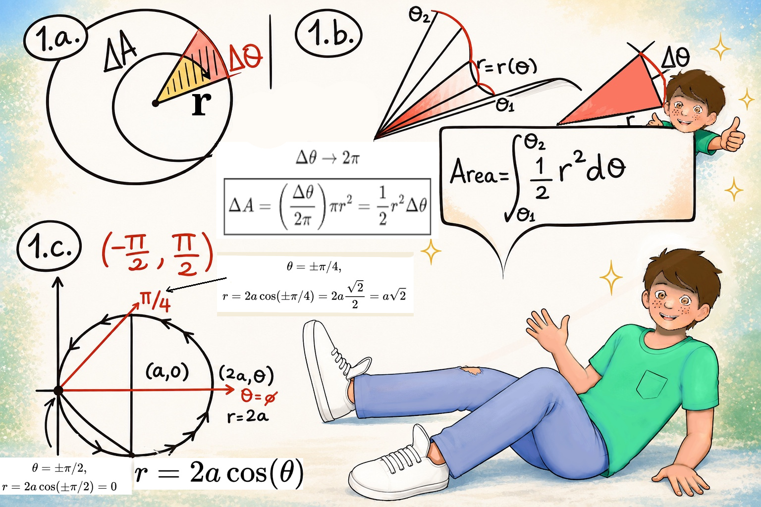
The circle with center (a, 0) and radius a, is described by the polar equation $r = 2a\cos(\theta)$. $(x-a)^2 + y^2 = a^2$, $\frac{-\pi}{2}< \theta < \frac{\pi}{2}$ (Figure 1.c.).

To trace the circle exactly once, we integrate from $\theta = -\frac{\pi}{2}$ to $\theta = \frac{\pi}{2}$ (since $\cos(\pm\frac{\pi}{2}) = 0$): $\text{Area} = \int_{-\pi/2}^{\pi/2} \frac{1}{2}(2a\cos(\theta))^2 \, d\theta = 2a^2 \int_{-\pi/2}^{\pi/2} \cos^2(\theta) \, d\theta$

Using the trigonometric half-angle identity $\cos^2(\theta) = \frac{1 + \cos(2\theta)}{2}$: $\text{Area} = 2a^2 \int_{-\pi/2}^{\pi/2} \frac{1 + \cos(2\theta)}{2} \, d\theta = a^2 \left[ \theta + \frac{1}{2}\sin(2\theta) \right]_{-\pi/2}^{\pi/2}$

Evaluating at the bounds (and noting that $\sin(\pi) = \sin(-\pi) = 0$): $\text{Area} = a^2 \left( \frac{\pi}{2} - \left(-\frac{\pi}{2}\right) \right) = \pi a^2$

This perfectly matches the geometric area of a circle with radius $a$. 😃

Bibliography

1. NPTEL-NOC IITM, Introduction to Galois Theory.
2. Algebra, Second Edition, by Michael Artin.
3. LibreTexts, Calculus. Abstract and Geometric Algebra, Abstract Algebra: Theory and Applications (Judson).
4. Field and Galois Theory, by Patrick Morandi. Springer.
5. Michael Penn, and MathMajor.
6. Contemporary Abstract Algebra, Joseph, A. Gallian.
7. YouTube’s Andrew Misseldine: Calculus. College Algebra and Abstract Algebra.
8. MIT OpenCourseWare 18.01 Single Variable Calculus, Fall 2007 and 18.02 Multivariable Calculus, Fall 2007.
9. Calculus Early Transcendentals: Differential & Multi-Variable Calculus for Social Sciences.