The Fundamental Theorems of Calculus and the MVT for Integrals

“If you hear a voice within you say ‘you cannot paint’, then by all means paint and that voice will be silenced,” Vincent van Gogh.

Antiderivatives

Antiderivatives are the inverse operation of derivatives and form the foundation of integral calculus.

Given a function $f(x)$, an antiderivative (also known as an indefinite integral), denoted as $F(x)$, is a function that can be differentiated to obtain the original function, i.e., $F'(x) = f(x)$; e.g., $3x^2 - 1$ is the derivative of $x^3 - x + 7$, which means $x^3 - x + 7$ is an antiderivative of $3x^2 - 1$.

Symbolically, the process of finding antiderivatives is called integration, and we write it as: $F(x) = \int f(x)dx$

The Fundamental Theorem of Calculus (Net Change Theorem)

The Fundamental Theorem of Calculus bridges the gap between derivatives and integrals.

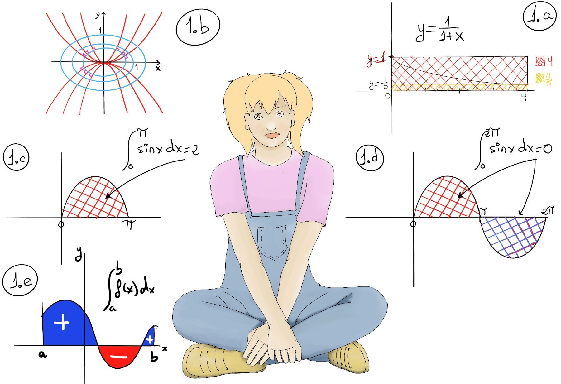
It states that the definite integral of a function $f$ over an interval $[a, b]$ is equal to the change in any of its antiderivatives $F$ between the ends of that interval: $\boxed{\int_{a}^{b} f(x)dx = F(b) - F(a) = F(x) \bigg\vert{}_{a}^{b}}$

If we consider $f$ to be a continuous rate of change (meaning $f(x) = F'(x)$), this theorem can be restated as the Net Change Theorem: The definite integral of a rate of change of a function on $[a, b]$ is the total change of the function itself on that interval.

Real-World Applications

• Average Velocity: Suppose a car moves along a straight road, and its position at time $t$ is $s(t)$. Its velocity is the derivative of position, $v(t) = s'(t)$. The average velocity over the time interval $[a, b]$ is the total change in position divided by the time elapsed:

$$\text{Average Velocity} = \frac{s(b)-s(a)}{b-a} = \frac{1}{b-a} \int_{a}^{b} v(t)dt$$

• Average Fluid Flow: Suppose water flows into a vessel at a rate of $1 - e^{-t} \text{ cm}^3/\text{s}$. The average rate of flow from $t = 0$ to $t = 2$ is:

$$\text{Average Flow} = \frac{1}{2-0}\int_{0}^{2} (1-e^{-t})dt = \frac{1}{2}(t + e^{-t})\bigg\vert{}_{0}^{2} = \frac{1}{2}(2 + e^{-2} - 1) \approx 0.56 \text{ cm}^3/\text{s}$$

The Average Value of a Function

Notice how the term $\frac{1}{b-a} \int_{a}^{b} f(x)dx$ appears frequently.

$\frac{f(b)-f(a)}{b-a} = \frac{\int_{a}^{b} f'(x)dx}{b-a}$ where the left side of this equation is just the average value of the function $f$ over the interval $[a, b]$.

The Mean Value Theorem for Integrals

If $f$ is a function that is continuous on $[a,b]$ and differentiable on $(a, b)$, then there is at least one point $c \in [a, b]$ such that $f(c) = \frac{1}{b-a}\int_{a}^{b} f(x)dx$ .

Geometrically, this means there is a rectangle with width $(b-a)$ and height $f(c)$ that has the exact same area as the region under the curve of $f(x)$ on that interval.

Proof.

1. Because $f$ is continuous on the closed interval $[a, b]$, the Extreme Value Theorem guarantees it has an absolute minimum $m$ and an absolute maximum $M$ on that interval.
   Therefore, for all $x \in [a, b]$: $m \le f(x) \le M$

2. By the Comparison Theorem for integrals, integrating all parts of this inequality yields: $m(b-a) \le \int_{a}^{b} f(x)dx \le M(b-a)$

3. Dividing everything by $(b-a)$, we see that the average value of the function is trapped between the absolute minimum and maximum: $m \le \frac{1}{b-a}\int_{a}^{b} f(x)dx \le M$

4. Because the average value is a number between $m$ and $M$, and $f$ is continuous, the Intermediate Value Theorem guarantees there must be some point $c \in [a, b]$ where $f(c)$ equals this average value. $\blacksquare$

The Second Fundamental Theorem of Calculus

While the first part of the Fundamental Theorem evaluates definite integrals, the second part allows us to construct antiderivatives from scratch using an “accumulation function.”

The Second Fundamental Theorem of Calculus. If $f$ is a continuous function and c is a constant, then f has a unique antiderivative A that satisfies $A(c) = 0$, and that antiderivative is given by the rule $A(x) = \int_{c}^{x} f(t)dt$.

Proof.

1. We start by using the limit definition of the derivative for $A(x)$: $A'(x) = \lim_{h \to 0} \frac{A(x+h) - A(x)}{h}$

2. $A'(x) = \lim_{h \to 0} \frac{\int_{c}^{x+h} f(t)dt - \int_{c}^{x} f(t)dt}{h}$

3. By the property of adjacent intervals ($\int_c^{x+h} = \int_c^x + \int_x^{x+h}$), we can simplify the numerator: $A'(x) = \lim_{h \to 0} \frac{\int_{x}^{x+h} f(t)dt}{h}$

4. By the Mean Value Theorem for Integrals (proven above), we know that for the interval $[x, x+h]$, there exists some number $c^*$ in that interval such that $\int_{x}^{x+h} f(t)dt = f(c^*) \cdot h$.
   $A'(x) = \lim_{h \to 0} \frac{f(c^*) \cdot h}{h} = \lim_{h \to 0} f(c^*)$

5. As $h$ approaches $0$, the interval $[x, x+h]$ shrinks to the single point $x$. Because $c^*$ is trapped inside this interval, $c^*$ is forced to approach $x$. Since $f$ is continuous, $\lim_{c^* \to x} f(c^*) = f(x)$.
   Therefore, $A'(x) = f(x) \quad \blacksquare$.

Solved exercises

• Suppose $F'(x) = \frac{1}{1+x}$ and $F(0) = 1$. The Mean Value Theorem implies that $A < F(4) < B$. Compute $A$ and $B$.

Solution (Using the Mean Value Theorem):

Because $F$ is continuous on $[0, 4]$ and differentiable on $(0, 4)$, there exists a $c \in (0, 4)$ such that: $F(4) - F(0) = F'(c)(4 - 0)$

By assumption $F(0) = 1$, $F(4) - 1 = \left(\frac{1}{1+c}\right) \cdot 4$

Since $c \in (0, 4)$, we can bound the value of the derivative. The maximum value of $\frac{1}{1+c}$ on this interval occurs at $c=0$, and the minimum occurs at $c=4$.

Therefore, $\frac{1}{1+4} < \frac{1}{1+c} < \frac{1}{1+0}$

Simplifying, $\frac{1}{5} < \frac{1}{1+c} < 1$

Multiply the entire inequality by $4$: $\frac{4}{5} < \left(\frac{1}{1+c}\right) \cdot 4 < 4$

Next, we substitute $F(4) - 1$ back into the middle of our expression: $\frac{4}{5} < F(4) - 1 < 4$

$\frac{9}{5} < F(4) < 5$. Therefore, $A = \frac{9}{5}$ and $B = 5$.

Suppose F’(x) = $\frac{1}{1+x}, F(0) = 1$, the MVT implies A < F(4) < B, could you compute A and B?

Similarly, it could be argued by the Fundamental Theorem of Calculus, F(4) -F(0) = $\int_{0}^{4} \frac{dx}{1+x}dx <[x = 0] \int_{0}^{4} dx = 4$ -this is the red rectangle, Figure 1.a.-. On the other hand, F(4) -F(0) = $\int_{0}^{4} \frac{dx}{1+x}dx >[x = 4] \int_{1}^{5} \frac{1}{5}dx = \frac{4}{5}$ -this is the yellow rectangle below, Figure 1.a.-, and we obtain the same result.

 

• Suppose a car moves along a straight road, and its position at time t is given by the function s(t). The average velocity of the object over the time interval [a, b] can be represented by the average rate of change of s(t) over that interval, $\text{AverageVelocity} = \frac{s(b)-s(a)}{b-a}$.

Denoting the velocity as v(t), $\text{AverageVelocity} = \frac{s(b)-s(a)}{b-a} = \frac{1}{b-a} \int_{a}^{b} v(t)dt = \frac{1}{b-a} \int_{a}^{b} s'(t)dt$

Note: If y = s(t) represents the position function, then v = s′(t) represents the instantaneous velocity.

• Find the average value of the function $f(x) = 8 -2x$ over the interval [0, 4] and find the value c such that f(c) equals this average.

First, calculate the average value of the function: $\text{AverageValue} = \frac{1}{4-0}\int_{0}^{4} (8-2x)dx = \frac{1}{4}·(8x-x^2)\bigg|_{0}^{4} = \frac{1}{4}·(8·4-16) = 4$.

Next, set the original function equal to this average value and solve for $c$: $f(c) = 4$

$8 - 2c = 4$. Simplify, $2c = 4 \implies c = 2$

Because $2$ is within the interval $[0, 4]$, it satisfies the Mean Value Theorem for Integrals.

 

• Find $\frac{d}{dx} \int_{1}^{x} \frac{1}{t^2} \, dt$.

1. Recall. The First Fundamental Theorem of Calculus states that if $f$ is continuous, and $A(x) = \int_{c}^{x} f(t) \, dt$, then $A'(x) = f(x)$.

2. Direct Application. Let $A(x) = \int_{1}^{x} f(t) \, dt$, where $f(t) = \frac{1}{t^2}$ and $c = 1$.
   By the First Fundamental Theorem of Calculus, the derivative is simply the integrand evaluated at $x$: $A'(x) = f(x) = \frac{1}{x^2}$

3. Verification by Integration.
   Let’s check this by evaluating the integral first, then differentiating: $A(x) = \int_{1}^{x} t^{-2} \, dt = \left[ -t^{-1} \right]_{1}^{x} = -\frac{1}{x} - (-1) = 1 - \frac{1}{x}$
   Now, taking the derivative of our result: $\frac{d}{dx} A(x) = \frac{d}{dx} \left( 1 - \frac{1}{x} \right) = \frac{1}{x^2} \quad \blacksquare$
   Note: Because $A(1) = \int_{1}^{1} f(t) \, dt = 0$, we know that $A(x)$ is the unique antiderivative of $f(x)$ that satisfies the initial condition $A(1) = 0$.

• Find $\frac{d}{dx} \int_{2}^{x} (\cos(t) - t) \, dt$.

1. Direct Application. Let $A(x) = \int_{2}^{x} (\cos(t) - t) \, dt$. Here, $f(t) = \cos(t) - t$ and $c = 2$.
   By the First Fundamental Theorem of Calculus: $A'(x) = f(x) = \cos(x) - x$

2. Verification by Integration.
   Evaluate the integral explicitly: $A(x) = \int_{2}^{x} (\cos(t) - t) \, dt = \left[ \sin(t) - \frac{1}{2}t^2 \right]_{2}^{x} = \left( \sin(x) - \frac{1}{2}x^2 \right) - \left( \sin(2) - 2 \right)$
   Now, differentiate with respect to $x$ (remembering that the expression $\sin(2) - 2$ is just a constant): $\frac{d}{dx} A(x) = \cos(x) - x \quad \blacksquare$
   Since A(2) = $\int_{2}^{2} f(t)dt = 0$, A is the only antiderivative of f for which A(2) = 0.

• Find $\frac{d}{dx} \int_{1}^{\sqrt{x}} \sin(t) \, dt$.

Because the upper limit is a function of $x$ (not just $x$), we must combine the FTC with the Chain Rule.

1. Let $u(x) = \sqrt{x}$ and $G(u) = \int_{1}^{u} \sin(t) \, dt$. Our function is the composition $F(x) = G(u(x))$.

2. By the Chain Rule, $\frac{d}{dx}[G(u(x))] = G'(u) \cdot u'(x)$.

3. By the FTC, $G'(u) = \sin(u)$.

4. The derivative of the inner function is $u'(x) = \frac{1}{2\sqrt{x}}$.

5. Substituting these pieces together: $\frac{d}{dx} \int_{1}^{\sqrt{x}} \sin(t) \, dt = \sin(u(x)) \cdot \frac{du}{dx} = \sin(\sqrt{x}) \cdot \left( \frac{1}{2\sqrt{x}} \right) = \frac{\sin(\sqrt{x})}{2\sqrt{x}}$

6. $\frac{d}{dx} \int_{1}^{\sqrt{x}} sin(t)dt$ =[$u(x)=\sqrt{x}, F(x)=\int_{1}^{u(x)} sin(t)d(t) = G∘u, G(x)=\int_{1}^{x} sin(t)d(t)$]. By the The Second Fundamental Theorem of Calculus and the Chain Rules, $\frac{d}{dx} \int_{1}^{\sqrt{x}} sin(t)dt = sin(u(x))·\frac{du}{dx} = sin(u(x))·(\frac{1}{2}x^{\frac{-1}{2}}) = \frac{sin(\sqrt{x})}{2\sqrt{x}}$

 

The Evaluation Theorem

Theorem: If $f$ is continuous over the interval $[a, b]$, and $F$ is any antiderivative of $f$ (meaning $F'(x) = f(x)$), then: $\boxed{\int_{a}^{b} f(x) \, dx = F(b) - F(a) = F(x) \bigg\vert{}_{a}^{b}}$

In other words, the definite integral of a function over an interval is equal to the net change of its antiderivative between the endpoints.

Proof:

1. Let $F$ be any valid antiderivative of $f$, meaning $F'(x) = f(x)$.
2. Let’s define a new accumulation function $G(x) = \int_{a}^{x} f(t) \, dt$.
3. By the First Fundamental Theorem of Calculus, we know $G'(x) = f(x)$.
4. Because $F'(x) = f(x)$ and $G'(x) = f(x)$, their derivatives are identical. Therefore, $F(x)$ and $G(x)$ can only differ by a constant $C$: $F(x) = G(x) + C$
5. Now, let’s evaluate the difference $F(b) - F(a)$: $F(b) - F(a) = (G(b) + C) - (G(a) + C) = G(b) - G(a)$
6. By our original definition of $G(x)$: $G(b) = \int_{a}^{b} f(t) \, dt$, $G(a) = \int_{a}^{a} f(t) \, dt = 0$
7. Substituting these back into our equation yields: $F(b) - F(a) =[5] G(b) - G(a) = \int_{a}^{b} f(x) \, dx - 0 = \int_{a}^{b} f(x) \, dx$

Bibliography

1. NPTEL-NOC IITM, Introduction to Galois Theory.
2. Algebra, Second Edition, by Michael Artin.
3. LibreTexts, Calculus. Abstract and Geometric Algebra, Abstract Algebra: Theory and Applications (Judson).
4. Field and Galois Theory, by Patrick Morandi. Springer.
5. Michael Penn, and MathMajor.
6. Contemporary Abstract Algebra, Joseph, A. Gallian.
7. YouTube’s Andrew Misseldine: Calculus. College Algebra and Abstract Algebra.
8. MIT OpenCourseWare 18.01 Single Variable Calculus, Fall 2007 and 18.02 Multivariable Calculus, Fall 2007.
9. Calculus Early Transcendentals: Differential & Multi-Variable Calculus for Social Sciences.