
|
 |

|
|
|
|
|
|
Science is a differential equation, religion is a boundary condition, Alan Turing.
There are no atheists in foxholes, there is no love without pain, no rainbow without rain, nor faith without hope, no success without sacrifice, no life without death, no roses without spines, and life has no meaning or purpose without God, JustToThePoint, Anawim, #justtothepoint.
Antiderivatives are the inverse operation of derivatives and form the foundation of integral calculus.
Given a function $f(x)$, an antiderivative (also known as an indefinite integral), denoted as $F(x)$, is a function that can be differentiated to obtain the original function, i.e., $F'(x) = f(x)$; e.g., $3x^2 - 1$ is the derivative of $x^3 - x + 7$, which means $x^3 - x + 7$ is an antiderivative of $3x^2 - 1$.
Symbolically, the process of finding antiderivatives is called integration, and we write it as: $F(x) = \int f(x)dx$
The Fundamental Theorem of Calculus bridges the gap between derivatives and integrals.
It states that the definite integral of a function $f$ over an interval $[a, b]$ is equal to the change in any of its antiderivatives $F$ between the ends of that interval: $\boxed{\int_{a}^{b} f(x)dx = F(b) - F(a) = F(x) \bigg\vert{}_{a}^{b}}$
If we consider $f$ to be a continuous rate of change (meaning $f(x) = F'(x)$), this theorem can be restated as the Net Change Theorem: The definite integral of a rate of change of a function on $[a, b]$ is the total change of the function itself on that interval.
The Second Fundamental Theorem of Calculus. If $f$ is a continuous function and c is a constant, then f has a unique antiderivative A that satisfies $A(c) = 0$, and that antiderivative is given by the rule $A(x) = \int_{c}^{x} f(t)dt$.
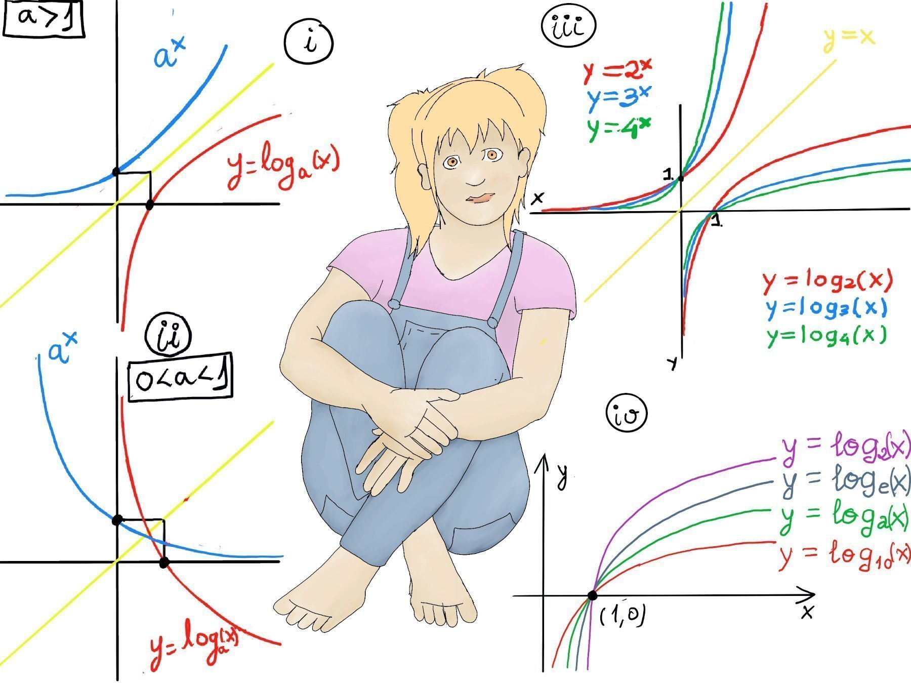
In algebra, the logarithm is introduced as the inverse function of exponentiation. We define the logarithm of a number $x$ to the base $a$ as the exponent $y$ to which $a$ must be raised to produce $x$: $\boxed{\log_a(x) = y \iff a^y = x}$
For example, $\log_4(64) = 3$ because $4^3 = 64$. $\log_2(16) = 4$ because $2^4=16$. $\log_8(512) = 3$ because $8^3=512$. However, $\log_2(-3)$ is undefined
Because any positive base raised to a real power is always positive, the logarithm’s domain is strictly all positive real numbers $(x > 0)$, while its range spans all real numbers $\mathbb{R}$. The graph of any standard logarithmic function passes through the $x$-intercept $(1, 0)$ (y-intercept: None), is one-to-one, and has a vertical asymptote along the y-axis at $x = 0$ (figures i and ii).
In calculus, the Power Rule for integration states that $\boxed{\int x^n \, dx = \frac{x^{n+1}}{n+1} + C}$. However, this rule breaks down completely when $n = -1$, leaving a gap in our mathematical toolkit: what is the antiderivative of $\frac{1}{x}$?
Instead of relying on algebraic exponents, we can use the Second Fundamental Theorem of Calculus to define the natural logarithm as an accumulation function.
Let us define a function $L(x)$ as the definite integral: $\boxed{L(x) = \int_{1}^{x} \frac{1}{t} \, dt} \quad \text{for } x > 0$.
Geometrically, $L(x)$ represents the exact area between the $x$-axis and the curve $y = \frac{1}{t}$ from $t = 1$ to $t = x$. From this single definition, all the familiar properties of the natural logarithm emerge naturally:

Using our integral definition, we can rigorously prove the algebraic rules of logarithms using standard integration techniques.
Let $a$ and $b$ be positive real numbers. We can split the integral of $L(ab)$ at $a$: $L(ab) = \int_{1}^{ab} \frac{1}{t} \, dt = \int_{1}^{a} \frac{1}{t} \, dt + \int_{a}^{ab} \frac{1}{t} \, dt$
The first integral is simply $L(a)$.
For the second integral, we apply integration by substitution.
Let $t = au$. This means the differential is $dt = a \, du$.
We also must adjust the bounds of integration:
$\star$ When $t = a$, $u = 1$.
$\star$ When $t = ab$, $u = b$.
Substituting these into the second integral: $\int_{a}^{ab} \frac{1}{t} \, dt = \int_{1}^{b} \frac{a \, du}{au} = \int_{1}^{b} \frac{1}{u} \, du = L(b)$
Therefore, $L(ab) = L(a) + L(b)$.
Using the definition: $L(a^r) = \int_{1}^{a^r} \frac{1}{t} \, dt$
We use substitution again. Let $w = t^{1/r}$, which means $t = w^r$.
The differential is $dt = r w^{r-1} \, dw$.
Adjusting the bounds:
$\star$ When $t = 1$, $w = 1$.
$\star$ When $t = a^r$, $w = a$.
Substituting these into the integral: $\int_{1}^{a^r} \frac{1}{t} \, dt = \int_{1}^{a} \frac{r w^{r-1} \, dw}{w^r} = \int_{1}^{a} \frac{r}{w} \, dw = r \int_{1}^{a} \frac{1}{w} \, dw = rL(a)$
The Second Fundamental Theorem of Calculus tells us that if $f$ is a continuous function, it has a unique antiderivative $A$ that satisfies $A(c) = 0$, given by the rule $A(x) = \int_{c}^{x} f(t) \, dt$.
Consider the differential equation $y' = e^{-x^2}$ with the initial condition $y(0) = 0$. The function $e^{-x^2}$ has no elementary antiderivative (it cannot be expressed using basic algebra, exponentials, or trigonometry). However, the equation y’ = $e^{-x^{2}}, y(0) = 0$ has a solution $\boxed{F(x) = \int_{0}^{x} e^{-t^2} \, dt}$ and c = 0 (F(0) = 0).
Even without an elementary formula, we can map the exact shape of $F(x)$ using its derivatives:
Slope: $F'(x) = e^{-x^2}$. Because $e$ raised to any power is positive, $F'(x) > 0$ for all real numbers. Thus, $F(x)$ is strictly increasing.
At the origin, the slope of the tangent line is $F'(0) = e^0 = 1$.
Concavity: The second derivative is $F''(x) = -2x e^{-x^2}$.
$\star$ When $x > 0$, $F''(x) < 0$ (concave down).
$\star$ When $x < 0$, $F''(x) > 0$ (concave up).
This means the function changes concavity exactly at the origin $(0,0)$, making it an inflection point.
Symmetry: Because the integrand $e^{-t^2}$ is an even function, $F(x)$ acts as an odd function. That means $F(-x) = -F(x)$, giving it rotational symmetry around the origin.
An even function satisfies: $e^{-(-t)^2} = e^{-t^2}$
Now compute F(-x), $F(-x) = \int_{0}^{-x} e^{-t^2} \, dt$
Reverse the limits using t = -u.
dt = -du; When t = 0, u = 0; When t = -x, u = x;
So: $F(-x) = \int_{0}^{-x} e^{-t^2} \, dt = \int_{0}^{x} e^{-(-u)^2} \, (-du) = -\int_{0}^{x} e^{-u^2} du = -F(x) \quad \blacksquare$
The plots shown below correspond to F and F'.
While the function $e^{-t^2}$ has no elementary antiderivative, advanced calculus techniques (specifically involving double integrals and polar coordinates) allow us to evaluate the total area under this Gaussian “bell curve” from $-\infty$ to $\infty$.
By integrating from the origin outward, the exact limits are: $\boxed{\lim_{x \to \infty} \int_{0}^{x} e^{-t^2} \, dt = \frac{\sqrt{\pi}}{2}}$ and $\boxed{\lim_{x \to -\infty} \int_{0}^{x} e^{-t^2} \, dt = -\frac{\sqrt{\pi}}{2}}$
Because this specific integral is foundational to probability, statistics, and partial differential equations (such as the heat equation), mathematicians standardized it into a special function known as the Gauss error function, denoted as $\text{erf}(x)$.
To make the function as clean and useful as possible, it is multiplied by a normalizing constant of $\frac{2}{\sqrt{\pi}}$. This scales the function so that its horizontal asymptotes sit perfectly at $1$ and $-1$.
The formal definition is as follows, $\boxed{\text{erf}(x) = \frac{2}{\sqrt{\pi}} \int_{0}^{x} e^{-t^2} \, dt}$.
By analyzing this integral definition and applying the Fundamental Theorem of Calculus, we can determine the exact behavior of the error function:
Domain: The function is defined for all real numbers $\mathbb{R}$.
Horizontal Asymptotes.
The normalization constant ensures the limits cap at exactly $1$ and $-1$.
$\lim_{x \to -\infty} (\frac{2}{\sqrt{\pi}}\int_{0}^{x} e^{-t^{2}}dt) = \frac{2}{\sqrt{\pi}}\int_{0}^{-\infty} e^{-t^{2}}dt = -\frac{2}{\sqrt{\pi}}\int_{-\infty}^{0} e^{-t^{2}}dt =$[This integral requires a more advanced knowledge of Calculus, $\int_{-\infty}^{0} e^{-t^{2}}dt = \frac{\sqrt{\pi}}{2}$] =$-\frac{2}{\sqrt{\pi}}·\frac{\sqrt{\pi}}{2} = -1$
$\lim_{x \to \infty} (\frac{2}{\sqrt{\pi}}\int_{0}^{x} e^{-t^{2}}dt) = \frac{2}{\sqrt{\pi}}\int_{0}^{\infty} e^{-t^{2}}dt =\frac{2}{\sqrt{\pi}}·\frac{\sqrt{\pi}}{2} = 1$
Therefore, the graph has two horizontal asymptotes: $y = 1$ and $y = -1$.
Monotonicity.
By the Second Fundamental Theorem of Calculus, the derivative of the error function is the integrand evaluated at $x$: $\text{erf}'(x) = \frac{2}{\sqrt{\pi}} e^{-x^2}$
Because $e^{-x^2}$ is strictly greater than $0$ for all real numbers, $\text{erf}'(x) > 0$ everywhere. This guarantees that the error function is constantly increasing.
Symmetry:
The error function is an odd function, meaning it possesses rotational symmetry around the origin: $\text{erf}(-x) = -\text{erf}(x)$
Because it is strictly increasing, bounded by horizontal asymptotes at $\pm 1$, and possesses odd symmetry, the graph of $\text{erf}(x)$ forms a classic sigmoid (S-shaped) curve.
It passes precisely through the origin $(0,0)$, where it crosses with its maximum slope of $\frac{2}{\sqrt{\pi}}$. This smooth, bounded shape is what makes it an essential tool for mapping cumulative probabilities in normal distributions across applied mathematics.

JustToThePoint Copyright © 2011 - 2026 Anawim. ALL RIGHTS RESERVED. Bilingual e-books, articles, and videos to help your child and your entire family succeed, develop a healthy lifestyle, and have a lot of fun. Social Issues, Join us.
This website uses cookies to improve your navigation experience.
By continuing, you are consenting to our
use of cookies, in accordance with our Cookies Policy and
Website Terms and Conditions of use.