Local Extrema

“Mr. Smith, could you explain to us what recursion is all about?” The professor in Introduction to Programming asked an apathetic student. “I don’t know the question, but sex, money, or both is definitely the answer, and God, justice, our values, and love are just the excuses,” I replied. “You shall not pass,” the teacher was far from amused, Apocalypse, Anawim, #justtothepoint.

Recall

Definition. A function f is a rule, relationship, or correspondence that assigns to each element x in a set D, x ∈ D (called the domain) exactly one element y in a set E, y ∈ E (called the codomain or range).

• The pair (x, y) is denoted as y = f(x) where: x is the independent variable (input) and y is the dependent variable (output). Often, both the domain D and codomain E are the set of real numbers ℝ or subsets of ℝ.

• D is the domain, the set of all possible inputs. E is the codomain or range, the set of all possible outputs.

• Key property💡: Each input has exactly one output. (No input is assigned two different outputs — this is the vertical line test!)

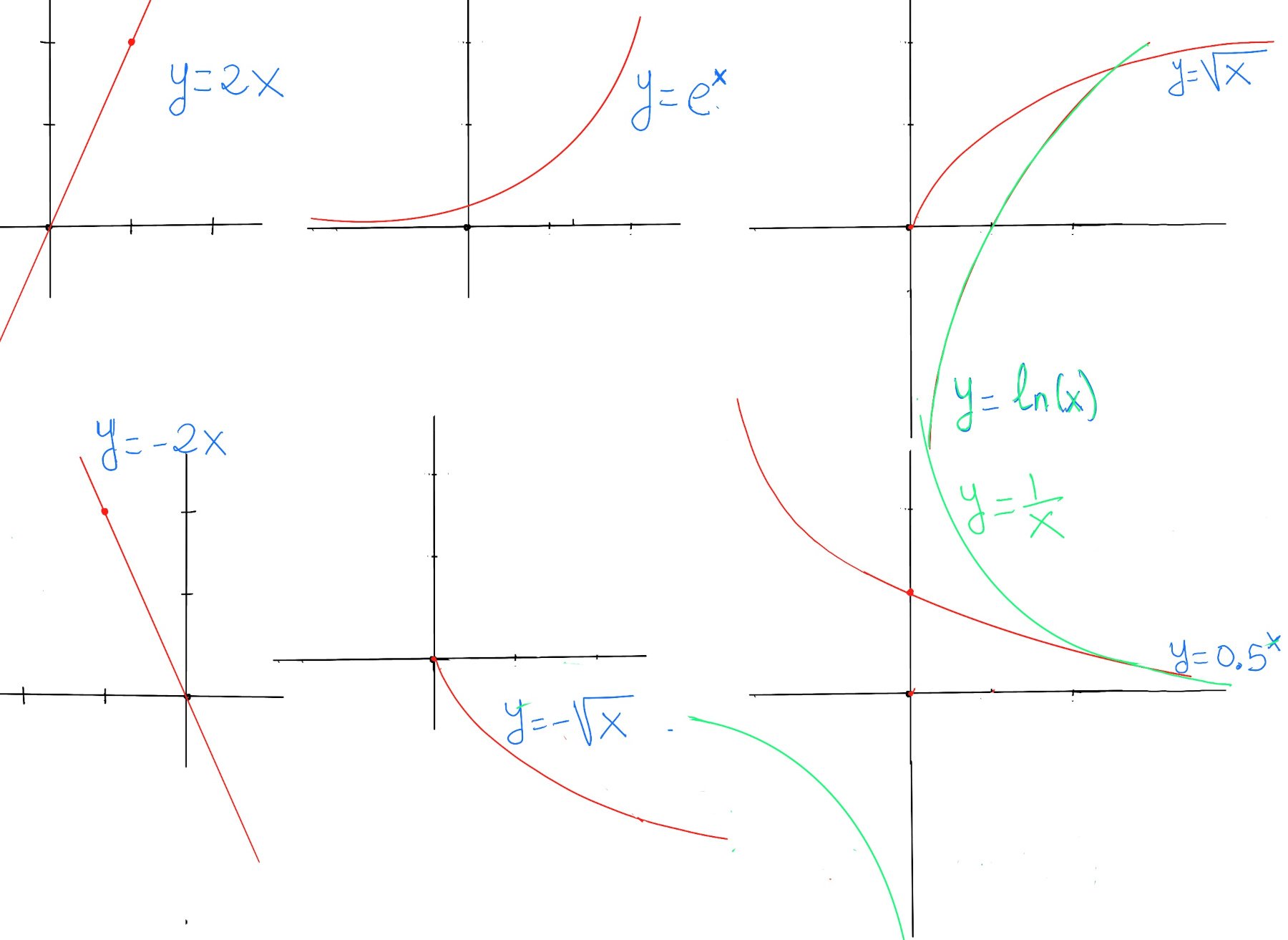
• Examples: constant, f(x) = c, horizontal line, slope = 0; linear, f(x) = mx + b, straight line, constant slope m and y-intercept b; quadratic $f(x) = ax^2 + bx + c$, u-shaped or inverted U, opens up (a > 0) or down (a < 0), vertex at x = $\frac{-b}{2a}$, symmetry about vertical axis through vertex; polynomial, $f(x) = a_n x^n + \dots + a_0$, a smooth and continuous curve, n roots (counting multiplicity), end behaviour determined by its leading term $a_n x^n$; exponential function, $f(x) = a \cdot b^x, a \ne 0, b \gt 0$, rapid growth (b > 1) or decay (0 < b < 1); trigonometric functions, $\sin(x), \cos(x), \tan (z)$ oscillatory, periodic behavior (period 2π for sin/cos, π for tan), sin and cos are bounded between -1 and 1, but tan is unbounded; step function $f(x) = \lfloor x \rfloor$, greatest integer ≤ x, constant on intervals [n, n+1), jumps at integers, its graph is a staircase shape; absolute value f(x) = |x|, V-shaped graph, slope changes at 0.

• Functions can be expressed in multiple forms, each useful in different contexts: verbal description, table of values (list of pairs), algebraic formula, graph, piecewise definition, recursive definition, parametric or integral form, and series representation.

• Evaluating a function means finding or computing the output value f(x) for a given input value x. f(x) = $x^2-2x +4, f(2) = 2^2 -2\cdot 2 + 4 = 4 - 4 + 4 = 4, f(0) = 0^2 -2\cdot 0 + 4 = 4, f(1) = 1^2 -2\cdot 1 + 4 = 1 -2 +4 = 3$

• The x-intercept is any point on the graph that intersects or crosses the x-axis. In other words, it is the value of x when the function (y-coordinate or y-value) is zero. The y-intercept is the point where the graph intersects or crosses the y-axis. y-coordinate of the point whose x-coordinate is 0, e.g., 2x - 3y = 6. x-intercept: set y = 0 → 2x = 6 ⇒ x=3, so (3, 0). y-intercept: set x = 0 → −3y = 6 ⇒ y = −2, so (0, −2).

A monotonic function is a mathematical function that maintains a consistent direction of change on its domain, either entirely increasing (monotonic increasing) or entirely decreasing (monotonic decreasing).

Let f be a function defined on some interval I. f increases on an interval I if f(b) >= f(a) ∀b > a, a,b ∈ I. If f(b) > f(a) ∀b > a, a, b ∈ I, the function is said to be strictly increasing on I.

Conversely, f decreases on an interval I if f(b) <= f(a) ∀b > a, a, b ∈ I. If f(b) < f(a) ∀b > a, a, b ∈ I, the function is said to be strictly decreasing. Finally, f is said to be constant on an interval I if f(a) = f(b) ∀a, b ∈ I.

Local Extrema

Local extrema are the largest or smallest values locally, that is, on an interval around the point. More formally, they are critical points on the graph of a function where the function reaches a maximum or minimum value (a valley) within a specific neighborhood of that point.

A critical point of a function f(x) occurs where the derivative f’(x) is either zero or undefined.

Definition. Let D be the domain of a function and c ∈ D. f is said to have a local or relative maximum point at c if there exists an interval (a, b) containing c such that f(c) is the maximum value of f on (a, b) ∩ D: f(c) ≥ f(x) ∀ x in (a, b) ∩ D.

Conversely, f is said to have a local or relative minimum point at c if there exists an interval (a, b) containing c such that f(c) is the minimum value of f on (a, b) ∩ D: f(c) ≤ f(x) ∀ x in (a, b) ∩ D.

A function has a local or relative extremum at c if c is either a relative maximum or minimum, that is, a point of the graph where f changes its monotonicity within the domain. Futhermore, a point of inflection is a point where the graph of f changes its concavity.

First Derivative Test. If the derivate f’(x) changes sign from positive to negative (as we look from read from left to right at the graph) at a critical point x = c, then f(c) is a local maximum (Figure 2.a)  

If the derivate f′(x) changes sign from negative to positive at a critical point x = c, then f(c) is a local minimum.

Proof.

Let’s confine ourself to the case of the minimum, the other case follows mutatis mutandis.

To the left from the point c, ∀x ∈ (c -δ, c), f’(x) < 0 ⇒[By Lagrange’s theorem, Let f be a function defined such that f: [a, b] → ℝ be a continuous function on [a, b] and differentiable on (a, b). Then, there exist some point c in this interval (a, b) such that the derivative of the function at the point c is equal to the difference of the function values at these points, divided by the difference of the point values, $f'(x_0)=\frac{f(b)-f(a)}{b-a}$] In this particular case, the difference of values of the function at the point x and c, f(x) - f(c) = f’(x₀)(x -c) [x, x₀ ∈ (c -δ, c) ⇒ f’(x₀) < 0, (x -c) < 0] f’(x₀)(x -c) > 0 ⇒ f(x) > f(c).

Analogously, ∀x ∈ (c, c + δ), f’(x) > 0 ⇒[By Lagrange’s Theorem] The difference of values of the function at the point x and c, f(x) - f(c) = f’(x₀)(x -c) [x, x₀ ∈ (c, c + δ) ⇒ f’(x₀) > 0, (x -c) > 0] f’(x₀)(x -c) > 0 ⇒ f(x) > f(c).

Second Derivative Test. If the first derivate of a function at a point c is zero (f'(c) = 0) and its exists the second derivate at this point and f''(c) > 0, then f(c) is a local minimum. Analogously, if f’(c) = 0 and f’’(c) < 0, then f(c) is a local maximum.

Proof.

Let’s confine ourself to the case of the minimum, the other case follows mutatis mutandis.

f’’(c) > 0 ⇒ The first derivate is increasing at this point c ⇒ ∃δ > 0: ∀x ∈ (c -δ, c), f’(x) < f’(c) = 0 and ∀x ∈ (c, c + δ), f’(x) > f’(c) = 0, and this is exactly the First Derivate Test.

Examples

• Calculate local maximum and minimum points for y = 2x² -5x + 3 (Figure 2.b), y’ = 4x -5. 0 = 4x -5, x = ⁵⁄₄ is a local (First Derivate Test) and a global minimum.

• Calculate local maximum and minimum points for y = ¹⁄₂x + sin(x) on [0, 2π] (Figure 2.c). y’ = ¹⁄₂ + cos(x), y’ = 0 ⇒ cos(x) = -¹⁄₂ ⇒ x = ^2π⁄₃, x = ^4π⁄₃. Local maximum ($\frac{2π}{3}, \frac{π}{3}+\frac{\sqrt{3}}{2}$) and local minimum ($\frac{4π}{3}, \frac{2π}{3}-\frac{\sqrt{3}}{2}$).

Calculate local maximum and minimum points for y = 3x⁵ -20x³ (Figure 2.d).

1. Let’s find the critical points by setting the derivate y’ = 15x⁴ -60x² to zero. 15x⁴ -60x² = 0 ↭ 15x²(x²-4) = 0. So, the critical points are x = 0, x = 2, and x = -2.
2. Use the second derivative test to determine the nature of each critical point and calculate local maximum and minimum points. y’’ = 60x³ -120x. y’’(0) = 0, y’’(2) > 0, and y’’(-2) < 0.

Therefore, it has a local minimum at x = 2 and a local maximum at x = -2. The critical point x = 0 is not a local extremum; it’s a point of inflection.

In the previous example (Figure 1), f has local or relative minimum points at -6, -3, and 7, and local or relative maximum points at -5, 0, and 4. On the open interval (0, 4), the function is constant, and therefore every point is both a local or relative maximum and minimum point. Futhermore, (-4, 0), (-2, 0), (0, 6), and (4, 6) are points of inflection.

Bibliography

1. NPTEL-NOC IITM, Introduction to Galois Theory.
2. Algebra, Second Edition, by Michael Artin.
3. LibreTexts, Calculus. Abstract and Geometric Algebra, Abstract Algebra: Theory and Applications (Judson).
4. Field and Galois Theory, by Patrick Morandi. Springer.
5. Michael Penn, and MathMajor.
6. Contemporary Abstract Algebra, Joseph, A. Gallian.
7. YouTube’s Andrew Misseldine: Calculus. College Algebra and Abstract Algebra.
8. MIT OpenCourseWare 18.01 Single Variable Calculus, Fall 2007 and 18.02 Multivariable Calculus, Fall 2007.
9. Calculus Early Transcendentals: Differential & Multi-Variable Calculus for Social Sciences.