Limits in Calculus

To be a star, you must shine your own light, follow your path, and don’t worry about the darkness, for that is when the stars shine brightest. Always do what you are afraid to do, Ralph Waldo.

Recall

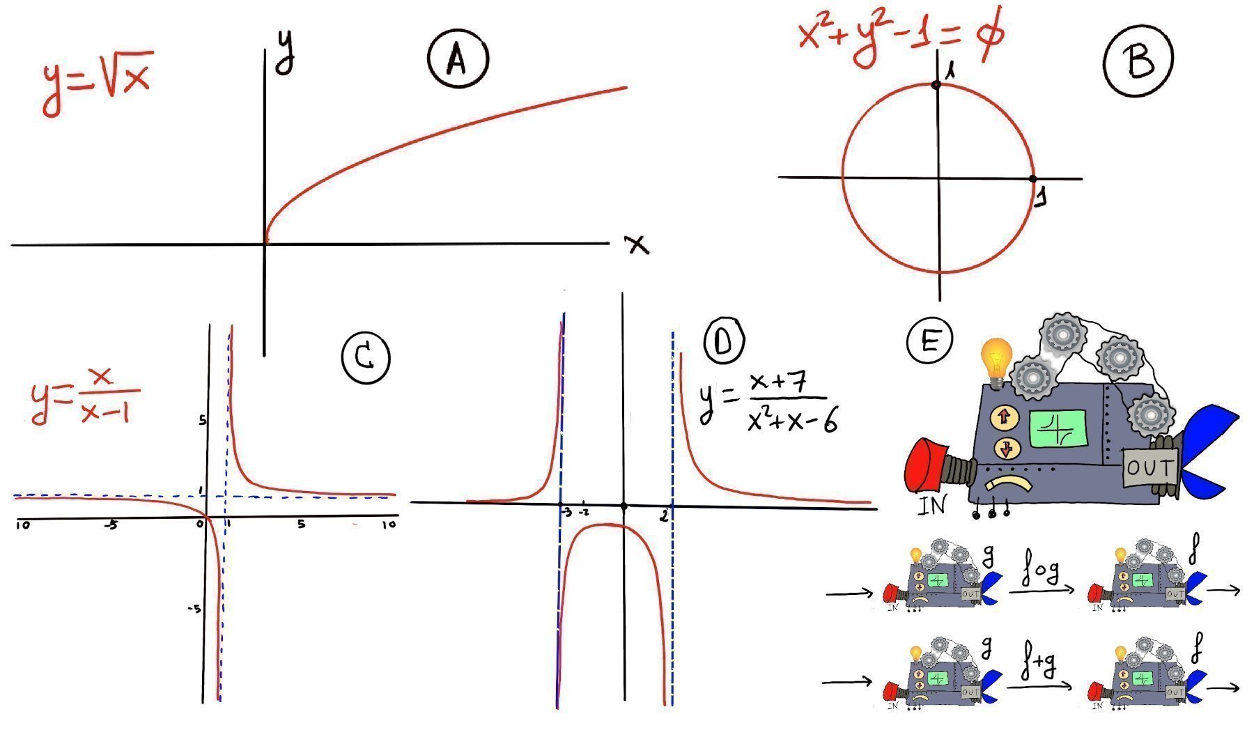
Definition. A function f is a rule, relationship, or correspondence that assigns to each element x in a set D, x ∈ D (called the domain) exactly one element y in a set E, y ∈ E (called the codomain or range).

• The pair (x, y) is denoted as y = f(x) where: x is the independent variable (input) and y is the dependent variable (output). Often, both the domain D and codomain E are the set of real numbers ℝ or subsets of ℝ. A mathematical function can be thought of as a black box (or machine) that takes an input from its domain and produces exactly one output in its codomain. Inside the machine lives a specific rule (formula, procedure, or mapping) that dictates or tells you which output corresponds to each input, and a key property is uniqueness —each input maps to a single, deterministic output. No input can ever produce two different results (Figure E). The function f(x) = x² accepts any real number x (domain: ℝ) and returns exactly one non-negative value x² (output in codomain: [0,∞)). The input 3 always yields 9, never any other value.

• D is the domain, the set of all possible inputs. E is the codomain or range, the set of all possible outputs.

• Key property💡: Each input has exactly one output. (No input is assigned two different outputs — this is the vertical line test!)

• Examples: constant, f(x) = c, horizontal line, slope = 0; linear, f(x) = mx + b, straight line, constant slope m and y-intercept b; quadratic $f(x) = ax^2 + bx + c$, u-shaped or inverted U, opens up (a > 0) or down (a < 0), vertex at x = $\frac{-b}{2a}$, symmetry about vertical axis through vertex; polynomial, $f(x) = a_n x^n + \dots + a_0$, a smooth and continuous curve, n roots (counting multiplicity), end behaviour determined by its leading term $a_n x^n$; exponential function, $f(x) = a \cdot b^x, a \ne 0, b \gt 0$, rapid growth (b > 1) or decay (0 < b < 1); trigonometric functions, $\sin(x), \cos(x), \tan (z)$ oscillatory, periodic behavior (period 2π for sin/cos, π for tan), sin and cos are bounded between -1 and 1, but tan is unbounded; step function $f(x) = \lfloor x \rfloor$, greatest integer ≤ x, constant on intervals [n, n+1), jumps at integers, its graph is a staircase shape; absolute value f(x) = |x|, V-shaped graph, slope changes at 0.

• Functions can be expressed in multiple forms, each useful in different contexts: verbal description, table of values (list of pairs), algebraic formula, graph, piecewise definition, recursive definition, parametric or integral form, and series representation.

• Evaluating a function means finding or computing the output value f(x) for a given input value x. f(x) = $x^2-2x +4, f(2) = 2^2 -2\cdot 2 + 4 = 4 - 4 + 4 = 4, f(0) = 0^2 -2\cdot 0 + 4 = 4, f(1) = 1^2 -2\cdot 1 + 4 = 1 -2 +4 = 3$

• The x-intercept is any point on the graph that intersects or crosses the x-axis. In other words, it is the value of x when the function (y-coordinate or y-value) is zero. The y-intercept is the point where the graph intersects or crosses the y-axis. y-coordinate of the point whose x-coordinate is 0, e.g., 2x - 3y = 6. x-intercept: set y = 0 → 2x = 6 ⇒ x=3, so (3, 0). y-intercept: set x = 0 → −3y = 6 ⇒ y = −2, so (0, −2).

• f is said to have a local or relative maximum at c if there exists an interval (a, b) containing c ($c \in (a, b)$) such that f(c) ≥ f(x) $∀ x \in (a, b) ∩ D$. f is said to have a local or relative minimum at c if there exists an interval (a, b) containing c ($c \in (a, b)$) such that f(c) ≤ f(x) $∀ x \in (a, b) ∩ D$.💡Local extrema can only occur where the function stops rising or falling —either because the derivative is zero, the derivative doesn't exist, or you're at the edge of the domain.

• First Derivative Test. Let f be differentiable on an open interval containing c, except possibly at c itself, and let c be a critical point (so f′(c) = 0 or f′ is undefined). Then:

1. If f′(x) > 0 for x just to the left of c and f′(x) < 0 for x just to the right of c, then f(c) is a local maximum.
2. If f′(x) < 0 for x just to the left of c and f′(x) > 0 for x just to the right of c, then f(c) is a local minimum.
3. If f′(x) does not change sign at c (stays positive or stays negative), then f(c) is not a local extremum.

• Second Derivative Test. If the first derivate of a function at a point c is zero (f'(c) = 0) and the second derivate at this point exists, then: (i) If f''(c) > 0, then f(c) is a local minimum. (ii) If f''(c) < 0, then f(c) is a local maximum. (iii) If f''(c) = 0, the test is inconclusive.
• Vertical asymptotes are vertical lines (perpendicular to the x-axis) of the form x = a (where a is a constant) near which the function grows without bound when x approaches a from at least one side. The line x = a is a vertical asymptote of f if at least one of the one-sided limits is infinite: $\lim_{x \to a^{-}}f(x)=\pm\infty$ or $\lim_{x \to a^{+}}f(x)=\pm\infty$.
• Horizontal asymptotes are horizontal lines (y = c, parallel to the x-axis) that the graph of the function approaches as x grows very large (positively or negatively). In other words, the function values get arbitrarily close to c as long as x is sufficiently large or more formally: $\lim_{x \to \infty}f(x)=c$ and/or $\lim_{x \to -\infty}f(x)=c$.
• A line y = m+b is an oblique (slant) asymptote as $x \to \infty$ if $\lim_{x\to\infty} [f(x) - (mx+b)] = 0.$ This means that the curve of f(x) gets more and more closer to the line y = mx + b as x grows large. For an asymptote y = mx + b as $x \to \infty, m = \lim_{x\to\infty} \frac{f(x)}{x}, b = \lim_{x\to\infty} \bigl(f(x) - m x\bigr)$, provided both limits exist.

Intuitive definition of a limit

Very loosing speaking, a limit is the value to which a mathematical function gets closer and closer to as the input gets closer and closer to some given value.

A limit describe what is happening around a given point, say “a”. It is the value that the function approaches as the input approaches “a”, and it does not depend on the actual value of the function at a, or even on whether the function is defined at “a” at all.

Limits are essential to calculus and mathematical analysis and the understanding of how functions behave. The concept of a limit can be written or expressed as $\lim_{x \to a} f(x) = L.$ This notation is read as “the limit of f as x approaches a equals L”.

Intuitively, this means that the values of f(x) can be made arbitrarily close to L (and I mean as close as we like, e.g., L ± 0.1, L ± 0.01, L ± 0.001, and so on), by choosing values of x sufficiently close to a, but not necessarily equal to a.

Consider the function f(x) = 2x² - 3x + 1. To compute or calculate $\lim_{x \to 2} 2x^2 -3x +1$, we observe that f is a polynomial, hence continuous. Therefore, the limit of f as x approaches 2 equals the value of the function at x = 2: $\lim_{x \to 2}(2x^2 -3x +1) = 2^2 -3\cdot 2 + 1 = 8 - 6 +1 = 3$.

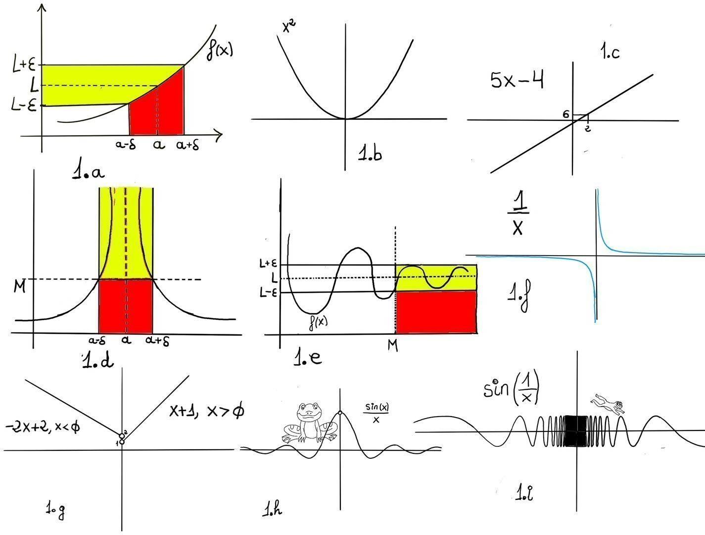
Similarly, $\lim_{x \to 0} x^2 = 0$ (Figure 1.b) and $\lim_{x \to 2} 5x -4 = 5·2 -4 = 6$ (Figure 1.c) because both functions are continuous everywhere.

Limits do not depend on the function value

Now consider the function $g(x) = \frac{x^2-1}{x-1}$. g(x) is a line, namely x + 1, but the function is undefined at x = 1, since division by zero is not allowed. In fact, Dom(g) = ℝ - {1}.

However, $\lim_{x \to 1} \frac{x^2-1}{x-1}$ =[If x ≠ 1 we can simplify] $\lim_{x \to 1} \frac{(x-1)(x+1)}{x-1} = \lim_{x \to 1} x +1 = 2.$ Even though the function is not defined at x = 1, the limit exists. In fact, the function is begging to be redefined as f(x) = x + 1, which would then be defined for all real numbers.

Piecewise-defined functions

Consider the function $f(x) = \begin{cases} 3x + 1, &x ≠ 2\\\\\\\\ 2, &x < 0 \end{cases}$

To calculate the limit $\lim_{x \to -2}$, we look at the expression used near x = 2, namely 3x + 1, so $\lim_{x \to -2} f(x) = \lim_{x \to -2} (3x + 1) = -6 +1 = -5.$ Notice that the value f(2) = 2 plays no role in the limit.

One-sided limits and nonexistence

Finally, let $f(x) = \begin{cases} -2x + 2, &x < 0 \\\\ x + 1, &x > 0 \end{cases}$ (Figure 1.g.)

Approaching 0 from the left (x < 0), f(x) becomes -2x + 2 and we get closer and closer to 2: $\lim_{x \to 0^-} f(x) = \lim_{x \to 0^-} -2x + 2 = 0$. Approaching 0 from the right (x > 0), f(x) becomes x + 1 and we get closer and closer to 1: $\lim_{x \to 0^+} f(x) = \lim_{x \to 0^+} x + 1 = 1$.

Since the left-hand and right-hand limits are different, the limit does not exist: $\lim_{x \to 1} f(x)$ does not exist because the left and right limits are not equal. A limit exists at a point if and only if both one-sided limits exist and are equal —regardless of whether the function is defined at that point.

How To Evaluate Limits From a Graph

When you evaluate a limit by looking at a graph you are asking: What value does f(x) get closer and closer to when x approaches a given point? The graph gives immediate visual clues — but you must be careful to check behaviour from both sides of the point, e.g., $\lim_{x \to 0} \frac{sin(x)}{x} = 1$

Given a graph of f and a point a:

1. Check the domain at a: is f(a) defined (solid dot), undefined (hole), or an asymptote (vertical line)? That obviously affects f(a) but not necessarily the limit.
2. Look from the left: follow the graph as x approaches “a” from values smaller than a. Does f(x) approach some finite number $L^-$, blow up to +∞ or −∞, or oscillate?
3. Look from the right: follow the graph as x approaches “a” from values bigger than a. Does f(x) approach some finite number $L^+$, blow up to +∞ or −∞, or oscillate?
4. Compute the limit. A limit exists at a point if and only if both one-sided limits exist and are equal —regardless of whether the function is defined at that point. (i) If $L^- = L^+ = L$ (finite), then $\lim_{x \to a}f(x) = L$. (ii) If $L^- = L^+ = +\infty$ or $L^- = L^+ = -\infty$, we say $\lim_{x \to a}f(x) = +\infty$ or $\lim_{x \to a}f(x) = -\infty$; strictly speaking the limit does not exist as a real number but this notation describes the blow-up behaviour of the function at a. (iii) If $L^-$ and $L^+$ differ, or if at least one of the one‑sided limits fails to exist, then the two-sided limit $\lim_{x \to a}f(x)$ does not exist.
5. Compare the limit with f(a). If $\lim_{x \to a}f(x)$ exists and equals f(a), f is continuous at a. If the limit exists but f(a) is different or undefined, the point is a removable discontinuity (a hole).

Examples and common graphical situations

1. $\lim_{x \to 0} \frac{sin(x)}{x} = 1$. Graphically (Figure 1.h), the curve $\frac{sin(x)}{x}$ approaches 1 from both sides as x approaches zero. The function is undefined at x = 0, but the limit exist and equals 1. Analytically this follows from: (i) $\forall x\in (0, \frac{\pi}{2}), cos(x) \le \frac{sin(x)}{x} \le 1$ (unit circle). Taking limits as $x \to 0, cos(x) \to 1$, and the constant 1 stays 1, so by the squeeze theorem, $\lim_{x \to 0} \frac{sin(x)}{x} = 1$; (ii) L’Hôpital’s rule, $\lim_{x \to 0} \frac{sin(x)}{x} = \lim_{x \to 0} \frac{cos(x)}{1} = cos(0) = 1$; (iii) Using the Taylor series: $sin(x) = x - \frac{x^3}{6} + \mathbb{O}(x^5) \implies \frac{sin(x)}{x} = 1 - \frac{x^2}{6} + \mathbb{O}(x^4)$. As $x\rightarrow 0$, all higher-order terms vanish, so: $\lim_{x \to 0} \frac{sin(x)}{x} = 1$.
2. Vertical asymptote at 0 for 1/x. $\lim_{x \to 0⁺} \frac{1}{x} = +∞$, $\lim_{x \to 0⁻} \frac{1}{x} = -∞$ (Figure 1.f). The right limit ($\lim_{x \to 0⁺} \frac{1}{x}$) means you approach the point x = 0 from the right, i.e., with values x bigger than 0. The left limit ($\lim_{x \to 0⁻} \frac{1}{x}$) means you approach the point x = 0 from the right, i.e., we must take values x lower than 0, hence $\lim_{x \to 0} \frac{1}{x}$ is undefined.
3. Oscillatory example: $\sin(\frac{1}{x})$ near 0 As $x \to 0, \sin(\frac{1}{x})$ oscillates wildly between -1 and 1 (infinitely often) and does not approach any single value. So $\lim_{x \to 0}\sin(\frac{1}{x})$ does not exist.
4. Removable discontinuity (hole). A function $f(x) = \frac{x^2-1}{x-1}$ that equals x + 1 everywhere except that it is undefined (a hole) at x = 1 still has $\lim_{x \to 1} f(x) = 2$. The graph shows a hole at (1, 2) but the left and right values approach 2.

Precise definition

We say that the limit of f, as x approaches a, is L, and write $\lim_{x \to a}f(x) = L$. For every real ε > 0, there exists a real δ > 0 such that whenever 0 < | x − a | < δ we have | f(x) − L | < ε. In other words, we can make f(x) arbitrarily close to L, f(x)∈ (L-ε, L+ε) (within any distance ε > 0) by making x sufficiently close to a (within some distance δ > 0, but not equal to a) (x ∈ (a-δ, a+δ), x ≠ a) -Fig 1.a.-

Graphically, one can draw a horizontal band (L − ε, L + ε) around L; there should exist a vertical interval or band (a − δ, a + δ) (punctured at or excluding a) such that the graph of f in that vertical strip (except possibly a) lies entirely inside the given horizontal band.

Alternative definition. Let f(x) be a function defined on an interval that contains x = a, except possibly at x = a, then we say that, $\lim_{x \to a} f(x) = L$ if $\forall \epsilon>0, \exists \delta>0: 0 < |x-a| <\delta \implies |f(x)-L|<\epsilon$

One-sided and infinite limits

Right-hand limit. $\displaystyle\lim_{x\to a^+} f(x)=L$ means that for every $\varepsilon>0$ there exists $\delta>0$ such that if $0 < x-a < \delta$ then $|f(x)-L| < \varepsilon$.

Left-hand limit. $\displaystyle\lim_{x\to a^-} f(x) = L$ means that for every $\varepsilon>0$ there exists $\delta>0$ such that if $0 < a-x < \delta$ then $|f(x)-L|<\varepsilon$.

Infinite limit. $\displaystyle\lim_{x\to a} f(x)=+\infty$ means that for every M > 0 there exists $\delta>0$ such that if $0 < |x-a| < \delta$ then f(x) > M, (Similar for $-\infty$.)

Solved easy exercises

• When direct substitution gives $\frac{0}{0}$ (an indeterminate form), the expression must be simplified first, e.g., $\lim_{x \to -2} \frac{x^2+x-2}{x+2} = \lim_{x \to -2} \frac{(x-1)(x+2)}{x+2} = \lim_{x \to -2} (x-1) = -3$.

  Finding a limit by factoring is a technique to computing limits that works by canceling out common factors. It allows us to transform an indeterminate form into one that allows for direct evaluation. Notice that the limit as x approaches -2 has nothing no to do with the value of the function at x = -2.

  $\lim_{x \to 2}\frac{x^2-4}{x-2} =\lim_{x \to 2}\frac{(x+2)(x-2)}{x-2} = \lim_{x \to 2}(x+2) = 4$
• If a function is continuous at the point (direct substitution), the limit equals the function value, e.g., $\lim_{x \to 4} x^{2} + x -11 =[\text{Polynomials are continuous everywhere, so:}] 4^2 + 4 - 11 = 9.$
• $\lim_{x \to 4} \frac {x + 3}{x^{2} + 12} =[\text{The denominator is not zero at x = 4, hence continuous}] \frac{7}{28} = 0.25.$
• Limits involving radicals (rationalization). Direct substitution gives $\frac{0}{0}$, so we rationalize the numerator. $\lim_{x \to 4} \frac{\sqrt{x}-2}{x-4} =[\text{Multiply numerator and denominator by the conjugate:}] \lim_{x \to 4} \frac{(\sqrt{x}-2)(\sqrt{x}+2)}{(x-4)(\sqrt{x}+2)} = \lim_{x \to 4} \frac{x-4}{(x-4)(\sqrt{x}+2)} = \lim_{x \to 4} \frac{1}{\sqrt{x}+2} = \frac{1}{4}.$
• $\lim_{x \to 0} \frac{x}{3-\sqrt{x+9}} =[\text{Rationalize the denominator:}] \lim_{x \to 0} \frac{x(3+\sqrt{x+9})}{(3-\sqrt{x+9})(3+\sqrt{x+9})} = \lim_{x \to 0} \frac{x(3+\sqrt{x+9})}{9-x-9} = \lim_{x \to 0} \frac{x(3+\sqrt{x+9})}{-x} = \lim_{x \to 0} -(3+\sqrt{x+9}) = -(3+3) = -6.$
• Limits of rational functions with common factors, e.g., $\lim_{x \to -2} \frac{x^2+5x+6}{x^2+6x+8} = [\text{Factor both numerator and denominator}]\lim_{x \to -2} \frac{(x+2)(x+3)}{(x+2)(x+4)} = \lim_{x \to -2} \frac{(x+3)}{(x+4)}=\frac{1}{2}.$
• Limits involving absolute value (one-sided limits), e.g, $\lim_{x \to 0}\frac{|x|}{x}$. Evaluate one-sided limits: $\lim_{x \to 0^-}\frac{|x|}{x} = \lim_{x \to 0^-}\frac{-x}{x} = -1, \lim_{x \to 0^+}\frac{|x|}{x} = \lim_{x \to 0^+}\frac{x}{x} = 1$. Since both one-sided limits exist but are not equal (-1 ≠ 1), the limit $\lim_{x \to 0}\frac{|x|}{x}$ do not exist. This is the canonical example of a function with a jump discontinuity at x = 0.

  A limit $\lim_{x \to a} f(x)$ exists iff both one-sided limits exist and are equal.

Bibliography

1. NPTEL-NOC IITM, Introduction to Galois Theory.
2. Algebra, Second Edition, by Michael Artin.
3. LibreTexts, Calculus.
4. Field and Galois Theory, by Patrick Morandi. Springer.
5. Michael Penn, and MathMajor.
6. Contemporary Abstract Algebra, Joseph, A. Gallian.
7. YouTube’s Andrew Misseldine: Calculus, College Algebra and Abstract Algebra.
8. Calculus Early Transcendentals: Differential & Multi-Variable Calculus for Social Sciences.
9. blackpenredpen.