The Limit Laws

If you torture data long enough, it will confess to anything or, in other words, there are different types of lies: white lies, seemingly small exaggerations and half-truths, damn lies, out-of-context information, and misleading statistics, #Anawim, justtothepoint.com.

Recall

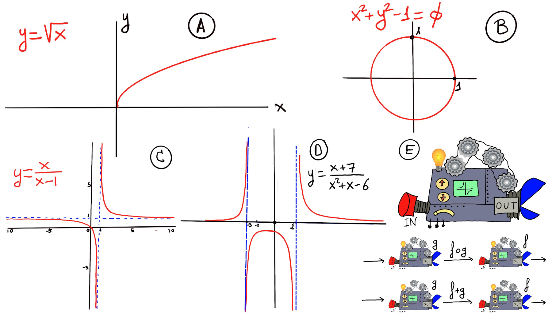
Definition. A function f is a rule, relationship, or correspondence that assigns to each element x in a set D, x ∈ D (called the domain) exactly one element y in a set E, y ∈ E (called the codomain or range). A mathematical function is like a black box that takes certain input values and generates corresponding output values (Figure E).

Very loosing speaking, a limit is the value to which a mathematical function gets closer and closer to as the input gets closer and closer to some given value.

A limit describe what is happening around a given point, say “a”. It is the value that the function approaches as the input approaches “a”, and it does not depend on the actual value of the function at a, or even on whether the function is defined at “a” at all.

Limits are essential to calculus and mathematical analysis and the understanding of how functions behave. The concept of a limit can be written or expressed as $\lim_{x \to a} f(x) = L.$ This notation is read as “the limit of f as x approaches a equals L”.

Intuitively, this means that the values of f(x) can be made arbitrarily close to L (and I mean as close as we like, e.g., L ± 0.1, L ± 0.01, L ± 0.001, and so on), by choosing values of x sufficiently close to a, but not necessarily equal to a.

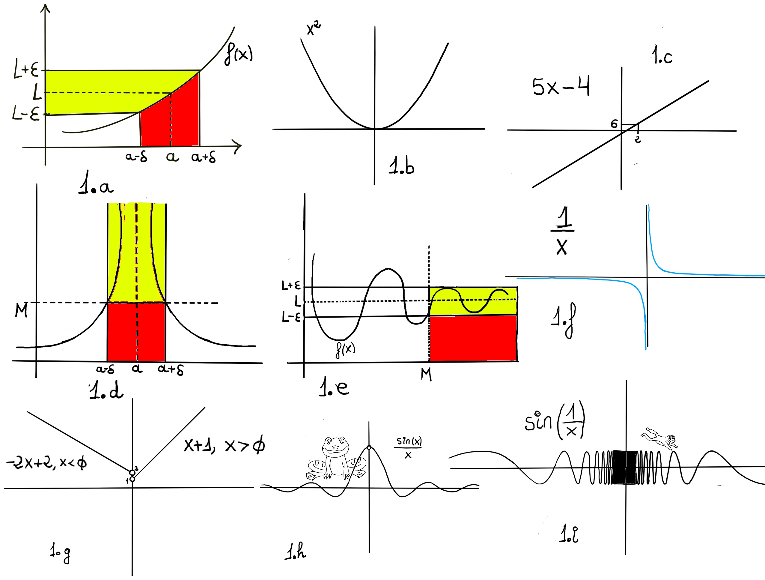
Formal definition. We say that the limit of f, as x approaches a, is L, and write $\lim_{x \to a}f(x) = L$. For every real ε > 0, there exists a real δ > 0 such that whenever 0 < | x − a | < δ we have | f(x) − L | < ε. In other words, we can make f(x) arbitrarily close to L, f(x)∈ (L-ε, L+ε) (within any distance ε > 0) by making x sufficiently close to a (within some distance δ > 0, but not equal to a) (x ∈ (a-δ, a+δ), x ≠ a) -Fig 1.a.-

The Limit laws

Let f(x) and g(x) be functions defined on an interval containing x = a, except possibly at x = a. Assume that the limits $ \lim_{x \to a} f(x) = L$ and $\lim_{x \to a} g(x) = M$ exist and are finite real numbers. Let c be a real constant. Under these assumptions, the following limit laws hold.

• Limit of a constant. The limit of a constant function is the constant itself, $\lim_{x \to a} k = k$ where k is a real number, e.g., $lim_{x \to 12} 7 = 7$. Formally, using the epsilon–delta definition: $\forall \epsilon \gt 0, \exist \delta \gt 0: 0 \lt |x - a| \lt \delta \text{ implies } | k - k| = 0 \lt \epsilon$, any $\delta$ would do (choose $\delta = \epsilon$ for simplicity).
• Sum law for limits. It states that the limit of the sum of two functions equals the sum of the limits of both functions, that is, $\lim_{x \to a} (f(x)+g(x)) = lim_{x \to a} f(x) + lim_{x \to a} g(x) = L + M,$ e.g., $lim_{x \to 2}(2x+7) = lim_{x \to 2}(2x) + lim_{x \to 2}(7) = 4+7 = 11.$

Proof: Let $\epsilon>0$

Since $lim_{x \to a} f(x) = L, \exists \delta_1>0: 0<|x-a|<\delta_1\, implies~ |f(x)-L|<\frac{\epsilon}{2}$

Since $lim_{x \to a} g(x) = M, \exists \delta_2>0: 0<|x-a|<\delta_2\, implies~ |g(x)-M|<\frac{\epsilon}{2}$

Let’s choose $\delta = \min(\delta_1, \delta_2).$

$\forall \epsilon>0, \exists \delta>0: 0<|x-a|<\delta$ ⇒[By the triangle inequality, |a + b| ≤ |a| + |b|] $|f(x)+g(x)-L-M| ≤ |f(x)-L|+ |g(x)-M| <\frac{\epsilon}{2} + \frac{\epsilon}{2} = \epsilon$

• Difference law for limits. It states that the limit of the difference of two functions equals the difference of the limits of both functions, that is, $\lim_{x \to a} (f(x)-g(x)) = lim_{x \to a} f(x) - lim_{x \to a} g(x) = L - M,$ e.g., $lim_{x \to 2}(2x-7) = lim_{x \to 2}(2x) - lim_{x \to 2}(7) = 4-7 = -3.$ This law follows directly from the sum (lim(f + g) = lim(f) + lim(g)) and constant multiple (lim(c⋅g) = c⋅ lim(g)) laws by writing f(x) − g(x) = f(x) + (−1)⋅g(x).

• Constant multiple law for limits. For any constant c, $\lim_{x \to a} c·f(x) = c·lim_{x \to a} f(x) = c·L,$ e.g., $\lim_{x \to 1} 7x^3 = 7·\lim_{x \to 1} x^3 = 7·1 = 7.$ Proof. We want to show that $\forall \epsilon>0, \exists \delta>0: 0<|x-a|<\delta, \text{ then } |cf(x) -cL| \lt \epsilon$.

  If c = 0, then |cf(x) -cL| = $|0 - 0| \lt \epsilon$ for any δ, so the limit is 0 = cL.

  If $c \ne 0, |cf(x) -cL| = |c|\cdot |f(x) -L| \lt |c|\cdot \frac{\epsilon}{|c|} = \epsilon$. Therefore, since $\lim_{x \to a} f(x) = L$, taken $\frac{\epsilon}{|c|} > 0$, there exist $\delta>0: 0<|x-a|<\delta, \text{ then } |f(x) -L| \lt \frac{\epsilon}{|c|}$.

• Product law for limits. It states that the limit of a product of two functions equals the product of the limits of both functions, that is, $\lim_{x \to a} (f(x)·g(x)) = lim_{x \to a} f(x) · lim_{x \to a} g(x) = L · M.$

$\lim_{x \to 2} x^2·(x+1) = \lim_{x \to 2} x^2·\lim_{x \to 2} x+1 = 4·3 = 12.$ $\lim_{x \to 2} (6x-x^3)·(x^2+3x-1) = \lim_{x \to 2} 6x-x^3·\lim_{x \to 2} x^2+3x-1 = 4·9 = 36.$ $\lim_{x \to 5} (2x^2-3x+4) = \lim_{x \to 5}(2x^2) - \lim_{x \to 5}(3x) + \lim_{x \to 5}(4) = 2·\lim_{x \to 5}(x^2) - 3·\lim_{x \to 5}(x) + \lim_{x \to 5}(4) = 2·5^2-3·5+4 = 39.$

Proof.

Let $\epsilon>0$

$\exists \delta>0: 0<|x-a|<\delta\, implies~ |f(x)g(x)-LM|<\epsilon$

|f(x)g(x)-LM| = |f(x)g(x) -Lg(x) + Lg(x) -LM| = |g(x)(f(x)-L) + L(g(x)-M)| ≤[Triangle inequality] |g(x)(f(x)-L)| + |L(g(x)-M)| = |g(x)||f(x)-L| + |L||g(x)-M|

This is the 🔑 tricky part:

1. $lim_{x \to a} g(x)$ = M ⇒ Let $\frac{ε}{2(|L|+1)}, \exists \delta_1>0: 0<|x-a|<\delta_1\, implies~ |g(x)-M|<\frac{ε}{2(|L|+1)}.$
2. Let $ε = 1> 0, \exists \delta_2>0: 0<|x-a|<\delta_2\, implies~ |g(x)-M|<1⇒|g(x)| = |g(x) -M +M| ≤ |g(x) -M| + |M|< 1 + |M|.$
3. $lim_{x \to a} f(x)$ = L ⇒ Let $\frac{ε}{2(|M|+1)}, \exists \delta_3>0: 0<|x-a|<\delta_3\, implies~ |f(x)-L|<\frac{ε}{2(|M|+1)}.$

We choose δ = min{δ₁, δ₂, δ₃}

|f(x)g(x)-LM| ≤ |g(x)||(f(x)-L)| + |L||(g(x)-M)| < $(1+|M|)\frac{ε}{2(|M|+1)}+|L|\frac{ε}{2(|L|+1)}<\frac{ε}{2}+|L|\frac{ε}{2|L|} = \frac{ε}{2}+\frac{ε}{2} = ε$∎

• Quotient law for limits. If $M \ne 0, \lim_{x \to a} \frac{f(x)}{g(x)} = \frac{\lim_{x \to a} f(x)}{\lim_{x \to a} g(x)} = \frac{L}{M}$, e.g., $\lim_{x \to 2} \frac{x^2-1}{x-1} = \frac{\lim_{x \to 2} x^2-1}{\lim_{x \to 2} x-1} = \frac{3}{1} = 3.$
• Power law for limits. It states that the limit of the nth power of a function equals the nth power of the limit of the function, that is, $\lim_{x \to a} (f(x))^{n} = (\lim_{x \to a} f(x))^{n} = L^{n}.$ Examples: $\lim_{x \to 5} (x+1)^{2} = (\lim_{x \to 5} x+1)^{2} = 6^{2} = 36$; $\lim_{x \to 2} (3x - 1)^4 = \left(\lim_{x \to 2} (3x-1)\right)^4 = 5^4 = 625$; $\lim_{x \to 3} \frac{1}{(x+1)^2} = \lim_{x \to 3} (x+1)^{-2} = 4^{-2} = \frac{1}{16}$; $\lim_{x \to 4} (x+5)^{1/2} = \left(\lim_{x \to 4} (x+5)\right)^{1/2} = 9^{1/2} = 3$; $\lim_{x \to -1} (x+2)^{2/3} = \left(\lim_{x \to -1} (x+2)\right)^{2/3} = 1^{2/3} = 1$; $\lim_{x \to 1} (x+3)^{\pi} = 4^{\pi} \approx 77.88$

Proof:

We proceed by induction on n.

1. Base case n = 1: $\lim_{x \to a} (f(x))^{1} = \lim_{x \to a} f(x) = L = L^1$.
2. Inductive step. Assume that $\lim_{x \to a} (f(x))^{k} = L^{k}$, for some positive integer k. Then, $\lim_{x \to a} (f(x))^{k+1} =[\text{By the product law for limits (since both limits exist)}] = (\lim_{x \to a} (f(x))^{k})\cdot (\lim_{x \to a} f(x)) = L^k\cdot L = L^{k+1}$. By induction, the power law holds for all positive integers n.
3. For negative integers n = -m (m > 0), if L ≠ 0, we have $\lim_{x \to a} (f(x))^{-m} = \lim_{x \to a} \frac{1}{f(x)^m} = \frac{1}{L^m} = L^{-m}$ using the power law for positive integers and the quotient law.
4. Let n=p/q or any real number. The function $g(y)=y^n$ is continuous on its domain (for L > 0 or appropriately restricted). By the continuity of the power function and the Limit of a Composite Function for continuous functions, $\lim_{x \to a}(f(x))^n = (\lim_{x \to a}f(x))^n = L^n$.

• Root law for limits. $\lim_{x \to a} \sqrt[n]{f(x)} = \sqrt[n]{\lim_{x \to a} f(x)} = \sqrt[n]{L} $ provided n is odd (no restriction on L) or n is even and L ≥ 0, e.g.,$\lim_{x \to 2} \sqrt{x^2+3x-1} = \sqrt{\lim_{x \to 2} x^2+3x-1} = \sqrt{9} = 3$ The Root Law is a special case of the Power Law with $n = \frac{1}{k}$: $\lim_{x \to a} \sqrt[n]{f(x)} = \lim_{x \to a}(f(x))^{\frac{1}{k}} = (\lim_{x \to a}f(x))^{\frac{1}{k}} = \sqrt[n]{\lim_{x \to a}f(x)} = \sqrt[n]{L}$ $\lim_{x \to 2} \sqrt[3]{\frac{5x+22}{2x}} = \sqrt[3]{\lim_{x \to 2} {\frac{5x+22}{2x}}} = \sqrt[3]{\frac{5·2+22}{2·2}} = \sqrt[3]{8} = 2.$
• Limit of a polynomial. Polynomials are continuous everywhere. This means that the limit of a polynomial as x approaches a is simply the polynomial evaluated at a. This follows from the basic limit laws: limits of sums, products, and constant multiples. $\lim_{x \to a} a_nx^n + a_{n-1}x^{n-1} + \ldots + a_2x^2 + a_1x + a_0 = a_n·a^n + a_{n-1}·a^{n-1} + \ldots + a_2·a^2 + a_1·a + a_0$, e.g., $\lim_{x \to 2} 3x^2-5x+7 = 3·2^2-5·2+7 = 12-10+7 = 9$.

1. Base case (n = 0). $P(x) = a_0$ is constant, so $\lim_{x \to a}a_0 = a_0 = P(a)$.
2. Inductive step. Assume the result holds for all polynomials of degree at most n −1. Consider $P(x) = a_nx^n + Q(x)$, where Q(x) is a polynomial of degree at most n - 1. We already know that (i) $\lim_{x \to a}x = a$ (identity function is continuous); (ii) By the power law for limits, $\lim_{x \to a}x^n = a^n$; (iii) By the constant multiple law, $\lim_{x \to a}a_nx^n = a_na^n$; (iv) By the inductive hypothesis, $\lim_{x \to a}Q(x) = Q(a)$.

Then by the sum law, $\lim_{x \to a}P(x) = \lim_{x \to a} (a_nx^n + Q(x)) = \lim_{x \to a}a_nx^n + \lim_{x \to a}Q(x) = a_na^n + Q(a) = P(a)$

• Limit of a composite function. The limit of a composition is the composition of the limit, provided the outside function is continuous at the limit of the inside function. $\lim_{x \to a} f ◦ g(x) = \lim_{x \to a} f(g(x)) = f(\lim_{x \to a} g(x))$ if f is continuous at $\lim_{x \to a} g(x).$ $\lim_{x \to 1} sin(\frac{π}{x+1}) = sin(\lim_{x \to 1} \frac{π}{x+1}) = sin(\frac{π}{2}) = 1.$ $\lim_{x \to 0} ln(cos(x)) = ln(\lim_{x \to 0} cos(x)) = ln(1)=$ [Recall e⁰ = 1] 0.
  $\lim_{x \to ∞} cos(\frac{1}{x}) = cos(\lim_{x \to ∞} \frac{1}{x}) = cos(0) = 1.$ $\lim_{x \to 0⁺} x^x = $[$e^{ln(x^x)}=e^{x·ln(x)}$] $\lim_{x \to 0⁺} e^{x·ln(x)} = e^{\lim_{x \to 0⁺} x·ln(x)} = e^{\lim_{x \to 0⁺} \frac{ln(x)}{\frac{1}{x}}}=$[ L’Hospital’s Rule] $e^{\lim_{x \to 0⁺} \frac{\frac{1}{x}}{\frac{-1}{x^2}}} = e^{\lim_{x \to 0⁺} -x} = e^0 = 1.$

Bibliography

1. NPTEL-NOC IITM, Introduction to Galois Theory.
2. Algebra, Second Edition, by Michael Artin.
3. LibreTexts, Calculus. Abstract and Geometric Algebra, Abstract Algebra: Theory and Applications (Judson).
4. Field and Galois Theory, by Patrick Morandi. Springer.
5. Michael Penn, Andrew Misseldine, and MathMajor, YouTube’s channels.
6. Contemporary Abstract Algebra, Joseph, A. Gallian.
7. MIT OpenCourseWare, 18.01 Single Variable Calculus, Fall 2007 and 18.02 Multivariable Calculus, Fall 2007, YouTube.
8. Calculus Early Transcendentals: Differential & Multi-Variable Calculus for Social Sciences.