
|
 |

|
|
|
|
|
|
Politicians are not born; they are excreted, Marcus Tullius Cicero.
Programming today is a race between software engineers striving to build bigger and better idiot-proof programs, and the Universe trying to produce bigger and better idiots. So far, the Universe is winning, Rick Cook, The Wizardry Compiled.
Let $f$ and $g$ be differentiable functions on an interval $I$, except possibly at a point $a$ contained in $I$. If $\lim_{x \to a} f(x) = \lim_{x \to a} g(x) = 0$ (or $\pm \infty$), and $g'(x) \neq 0$ for all $x \in I$ (except possibly at $a$), then: $\boxed{\lim_{x \to a} \frac{f(x)}{g(x)} = \lim_{x \to a} \frac{f'(x)}{g'(x)}}$, and that works provided that the limit on the right-hand side actually exists or equals $\pm \infty$.
This is the second article in our two-part series about the L’Hôpital’s Rule and is a continuation of the first one, so if you haven’t taken a look at it yet, I recommend you read it first and then, come back.
These are the most standard applications of L’Hôpital’s Rule. When you plug in the limiting value, you get exactly what the rule was built for: $\frac{\infty}{\infty}$ or $\frac{0}{0}$.
Rational Functions at Infinity. $\lim_{x \to ∞} \frac{x^2-9x+4}{3x^2+7x+8} = $
This is an indeterminate form of type $\frac{\infty}{\infty}$. Apply, L’Hôpital’s Rule = $\lim_{x \to ∞} \frac{2x-9}{6x+7} =$
The limit is still $\frac{\infty}{\infty}$, so apply L’Hôpital’s Rule again: $ = \lim_{x \to ∞} \frac{2}{6} = \frac{1}{3}.$
💡 Pro Tip: For rational functions where the degree of the numerator equals the degree of the denominator (here, both are $x^2$), the limit at infinity is simply the ratio of the leading coefficients: $\frac{1}{3}$.
Algebraic Manipulation First. $\lim_{x \to 0} \frac{x-\sin(x)}{x-\tan(x)}$
Direct substitution yields $\frac{0}{0}$. Let’s apply L’Hôpital’s Rule:
$= \lim_{x \to 0} \frac{1-\cos(x)}{1-\sec^2(x)}$
This still yields $\frac{0}{0}$. We could use L’Hôpital’s again, but the derivatives will get messy.
Instead, let’s use algebra. Multiply the numerator and denominator by $\cos^2(x)$: $= \lim_{x \to 0} \frac{(1-\cos(x))\cos^2(x)}{(1-\sec^2(x))\cos^2(x)} [\sec^2(x)\cos^2(x) = \frac{1}{\cos^2(x)}\cdot \cos^2(x) = 1] \lim_{x \to 0} \frac{(1-\cos(x))\cos^2(x)}{\cos^2(x)-1}$
Now, factor the difference of squares in the denominator: $\cos^2(x)-1 = (\cos(x)-1)(\cos(x)+1)$. Notice that $\cos(x)-1$ is the negative of $1-\cos(x)$. Therefore, $= \lim_{x \to 0} \frac{(1-\cos(x))\cos^2(x)}{-(1-\cos(x))(\cos(x)+1)} = \lim_{x \to 0} \frac{\cos^2(x)}{-(\cos(x)+1)}$
Now we can evaluate safely: $= \frac{1^2}{-(1+1)} = -\frac{1}{2}$
Advanced Factoring. $\lim_{x \to 2^+} \frac{\ln(x^3-8)}{\ln(x^2-3x+2)}$. The reader should notice that we need to use $2^+$ because the domain of the natural log requires positive arguments.
Direct substitution yields $\frac{-\infty}{-\infty}$. Apply L’Hôpital’s Rule: $= \lim_{x \to 2^+} \frac{\frac{3x^2}{x^3-8}}{\frac{2x-3}{x^2-3x+2}} = \lim_{x \to 2^+} \frac{3x^2(x^2-3x+2)}{(x^3-8)(2x-3)}$
Before blindly deriving again, let’s factor. Recall that $a^3-b^3 = (a-b)(a^2+ab+b^2)$, so $x^3-8 = (x-2)(x^2+2x+4)$
$= \lim_{x \to 2^+} \frac{3x^2(x-1)(x-2)}{(x-2)(x^2+2x+4)(2x-3)}$
Cancel the $(x-2)$ terms to remove the singularity: $= \lim_{x \to 2^+} \frac{3x^2(x-1)}{(x^2+2x+4)(2x-3)} = \frac{3(4)(1)}{(4+4+4)(4-3)} = \frac{12}{12} = 1$
Before we tackle the next set, look at the graph below. Notice how the red polynomial curves might start out strong, but the blue exponential curve always violently overtakes them eventually.
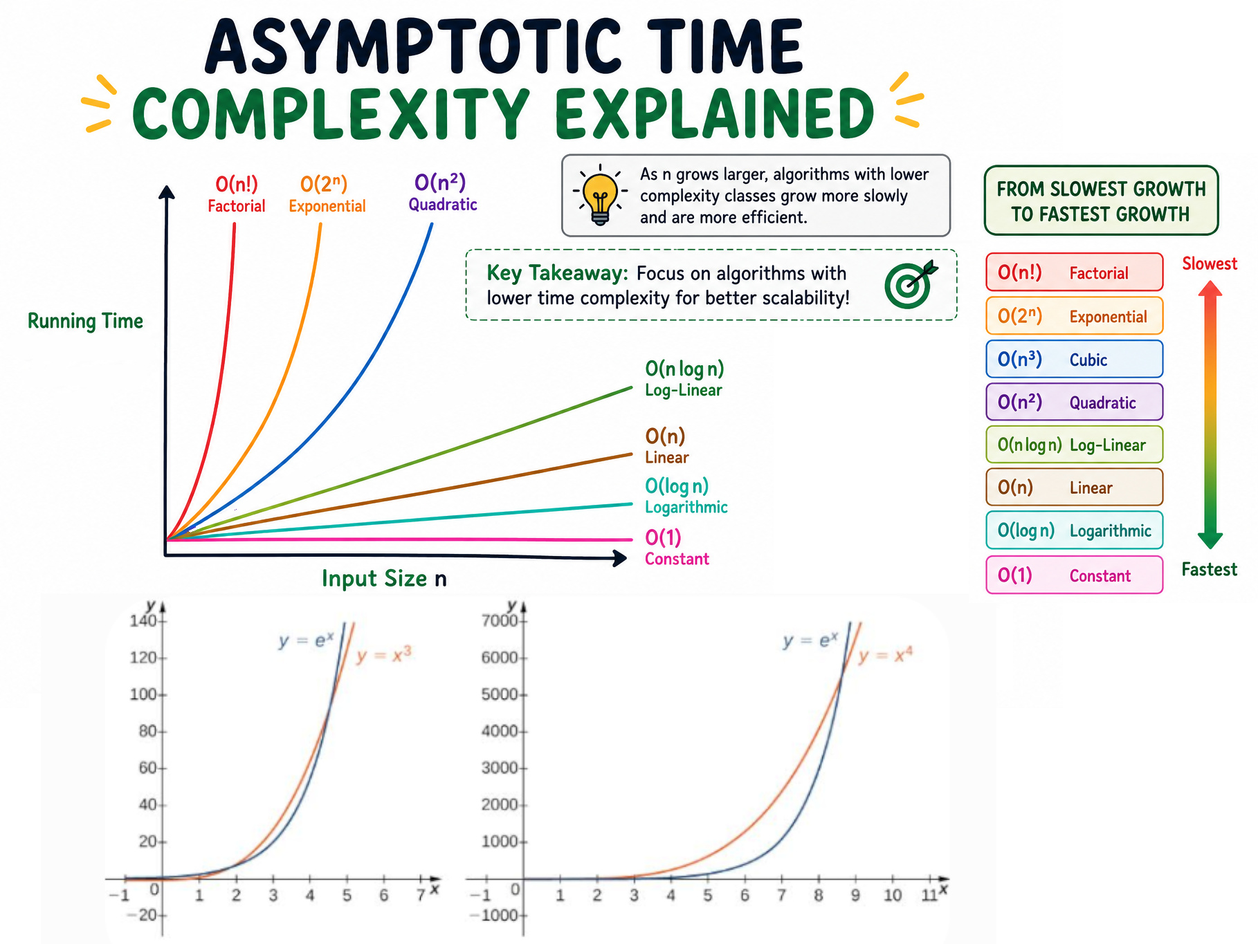
When evaluating limits to infinity, remember this Hierarchy of Growth: Logarithms $\ll$ Polynomials (Roots/Powers) $\ll$ Exponentials
L’Hôpital’s Rule algebraically confirms what the hierarchy tells us intuitively.
Root vs. Exponential. $\lim_{x \to \infty} \frac{\sqrt{x}}{e^x}$
Form: $\frac{\infty}{\infty}$. Applying L’Hôpital’s Rule: $= \lim_{x \to \infty} \frac{\frac{1}{2\sqrt{x}}}{e^x} = \lim_{x \to \infty} \frac{1}{2\sqrt{x}e^x} = 0$
Intuition: The exponential denominator grows vastly faster than the square root numerator -Exponential functions $e^x$ grow significantly faster than any power function $\sqrt{x}, x, x^2, \cdots$-, driving the fraction to zero.
Logarithm vs. Root. $\lim_{x \to \infty} \frac{\ln(x)}{x^{1/3}}$
Form: $\frac{\infty}{\infty}$. Applying L’Hôpital’s Rule: $= \lim_{x \to \infty} \frac{\frac{1}{x}}{\frac{1}{3}x^{-2/3}} = \lim_{x \to \infty} 3x^{(2/3 - 1)} = \lim_{x \to \infty} 3x^{-1/3} = \lim_{x \to \infty} \frac{3}{x^{1/3}} = 0$
Intuition: $\ln(x)$ grows slower than $x^{1/3}$ (or any arbitrary positive power of $x$). Logarithms are the slowest-growing mathematical functions we commonly encounter.
Exponentials vs. Any Power. Let $a > 1$. $\lim_{x \to \infty} \frac{e^{px}}{x^a}$
We can rewrite this limit to pull the exponent $a$ out: $= \left( \lim_{x \to \infty} \frac{e^{px/a}}{x} \right)^a$
Now apply L’Hôpital’s to the inside ($\frac{\infty}{\infty}$): $= \left( \lim_{x \to \infty} \frac{\frac{p}{a} e^{px/a}}{1} \right)^a = (\infty)^a = \infty$
Intuition: The exponential $e^{px}$ grows faster than any power of $x$ as $x \to \infty$, no matter how big, or even massive, the power $a$ is — the polynomial wins early, but the exponential always takes the lead eventually.
You cannot apply L’Hôpital’s Rule directly to $0 \cdot \infty$. You must force it into a fraction by rewriting one of the terms as its reciprocal: $A \cdot B = \frac{A}{(1/B)}$.
The Polynomial and the Negative Exponential. $\lim_{x \to -\infty} x^2e^x$
Direct evaluation gives $\infty \cdot 0$. To use L’Hôpital, move the exponential to the denominator by negating its exponent: $= \lim_{x \to -\infty} \frac{x^2}{e^{-x}}$
Now we have $\frac{\infty}{\infty}$. Apply L’Hôpital’s twice: $= \lim_{x \to -\infty} \frac{2x}{-e^{-x}} \quad \xrightarrow{L'H} \quad = \lim_{x \to -\infty} \frac{2}{e^{-x}} = 0$
Intuition: As $x$ approaches negative infinity, $x^2$ approaches positive infinity, but at a decreasing rate compared to the shrinking $e^x$.
The General Case. Let $a > 0$. $\lim_{x \to \infty} xe^{-ax}$
Direct evaluation gives $\infty \cdot 0$. Rewrite as a fraction: $= \lim_{x \to \infty} \frac{x}{e^{ax}}$
Apply L’Hôpital’s ($\frac{\infty}{\infty}$): $= \lim_{x \to \infty} \frac{1}{ae^{ax}} = \frac{1}{\infty} = 0$
These are the most complex indeterminate forms.
💣 Warning: $1^\infty$ does not equal 1. For example, $\lim_{n \to \infty} (1+\frac{1}{n})^n = e \approx 2.71828$.
The universal trick for exponent limits is to rewrite $f(x)^{g(x)}$ using the property $e^{\ln(y)} = y$. This allows you to bring the troublesome exponent down into a multiplication format.
$0^0$, $\lim_{x \to 0^+} x^x$
First, rewrite using the exponential/logarithm trick: $\lim_{x \to 0^+} x^x = \lim_{x \to 0^+} e^{\ln(x^x)} = \lim_{x \to 0^+} e^{x\ln(x)}$
Because $e^x$ is continuous, we can move the limit up into the exponent: $\lim_{x \to 0^+} e^{x\ln(x)} = e^{\lim_{x \to 0^+} x\ln(x)}$. Let’s solve just that exponent limit, which is now a $0 \cdot -\infty$ form: $\lim_{x \to 0^+} x\ln(x) = \lim_{x \to 0^+} \frac{\ln(x)}{1/x}$
Apply L’Hôpital’s to this new $\frac{-\infty}{\infty}$ form: $= \lim_{x \to 0^+} \frac{1/x}{-1/x^2} = \lim_{x \to 0^+} (-x) = 0$
Finally, plug this back into our base $e$: $\lim_{x \to 0^+} x^x = e^0 = 1$
$\infty^0$, $\lim_{x \to \infty} x^{\frac{1}{x}}$
Rewrite using the exponential/logarithm trick: $\lim_{x \to \infty} x^{\frac{1}{x}} = \lim_{x \to \infty} e^{\ln(x^{\frac{1}{x}})} = \lim_{x \to \infty} e^{\frac{\ln(x)}{x}}$
Focus on the exponent limit ($\frac{\infty}{\infty}$) and apply L’Hôpital’s: $\lim_{x \to \infty} \frac{\ln(x)}{x} \quad \xrightarrow{L'H} \quad \lim_{x \to \infty} \frac{1/x}{1} = 0$
Plug it back in: $\lim_{x \to \infty} x^{\frac{1}{x}} = e^0 = 1$.
$1^\infty$. The Tricky Negative, $\lim_{x \to \infty} \left(1-\frac{1}{x}\right)^x$
Rewrite using the exponential/logarithm trick: $\lim_{x \to \infty} \left(1-\frac{1}{x}\right)^x = e^{\lim_{x \to \infty} \ln\left((1-\frac{1}{x})^x\right)} = e^{\lim_{x \to \infty} x\ln\left(1-\frac{1}{x}\right)}$
To fix the $\infty \cdot 0$ in the exponent, drop $x$ to the denominator as $x^{-1}$: $\lim_{x \to \infty} \frac{\ln(1-\frac{1}{x})}{\frac{1}{x}}$
Now apply L’Hôpital’s ($\frac{0}{0}$): $= \lim_{x \to \infty} \frac{\left(\frac{1}{1-\frac{1}{x}}\right)\cdot\left(\frac{1}{x^2}\right)}{\frac{-1}{x^2}}$
The $\frac{1}{x^2}$ terms cancel cleanly! $= \lim_{x \to \infty} \frac{-1}{1-\frac{1}{x}} = \frac{-1}{1-0} = -1$
Plug this limit back into the base: $\lim_{x \to \infty} \left(1-\frac{1}{x}\right)^x = e^{-1} = \frac{1}{e}$
Complex $1^\infty$ Trigonometry, $\lim_{x \to 0} (\cos(x))^{\frac{1}{x^2}}$
Rewrite using the exponential/logarithm trick: $\lim_{x \to 0} (\cos(x))^{\frac{1}{x^2}} = e^{\lim_{x \to 0} \frac{\ln(\cos(x))}{x^2}}$
Evaluate the exponent ($\frac{0}{0}$): $\lim_{x \to 0} \frac{\ln(\cos(x))}{x^2}$
Apply L’Hôpital’s rule: $= \lim_{x \to 0} \frac{\frac{1}{\cos(x)} \cdot (-\sin(x))}{2x} = \lim_{x \to 0} \frac{-\tan(x)}{2x}$
This is still $\frac{0}{0}$. Apply L’Hôpital’s one last time: $= \lim_{x \to 0} \frac{-\sec^2(x)}{2} = \frac{-1}{2}$
Plug the limit back into the base: $\lim_{x \to 0} (\cos(x))^{\frac{1}{x^2}} = e^{-\frac{1}{2}} = \frac{1}{\sqrt{e}}$
When analyzing the running time or space usage of algorithms, we cannot simply measure the time in seconds, because that depends heavily on hardware, the operating system, and the programming language. Instead, we estimate the time or space as a function of the input size.
For example, when analyzing an algorithm that sorts a list of numbers, we evaluate how the number of primitive operations (lines of code executed) scales as the length of the input list ($n$) grows.
In mathematics and computer science, rates of growth (asymptotic growth) refer to the asymptotic behavior of functions as their input values become very large.
Formally, we express that a function $f(x)$ grows strictly slower than a function $g(x)$ using “little-o” notation or the $\ll$ symbol. This means that as the input approaches infinity, $g(x)$ dominates $f(x)$: $\boxed{\lim_{x \to \infty}\frac{f(x)}{g(x)} = 0}$
For example, as $x \to \infty$ and $p > 0$: $1 \ll \log_2(x) \ll x \ll x\log_2(x) \ll x^2$, $\ln(x) \ll x^p \ll e^x \ll e^{x^2}$
Analogously, for inverse functions: $\frac{1}{\ln(x)} \gg \frac{1}{x^p} \gg e^{-x} \gg e^{-x^2}$
While limits describe precise mathematical relationships, computer science typically relies on three specific notations to classify how execution time or space requirements grow:
In asymptotic analysis, constant factors and lower-order terms become virtually meaningless in the face of an arbitrarily large $n$. Therefore, they are dropped.
An algorithm that takes $7n + 15$ operations is simply classified as $O(n)$. Because $n$ drives the growth, a linear algorithm with a massive constant factor will still eventually outperform a quadratic algorithm with a tiny constant factor as the data scales.
Asymptotic growth is categorized into several standard complexity classes, ordered below from fastest/most efficient to slowest/least efficient:
| Complexity Class | Notation | Description | Example Algorithm |
|---|---|---|---|
| Constant | $O(1)$ | Execution time is independent of input size. | Accessing an array by index. |
| Logarithmic | $O(\log n)$ | Execution time grows very slowly as input increases. | Binary search in a sorted list. |
| Linear | $O(n)$ | Execution time grows directly in proportion to the input. | Finding the maximum value in an unsorted list. |
| Linearithmic | $O(n \log n)$ | Slightly worse (slower) than linear, typical of efficient sorting algorithms. | Merge Sort, Quick Sort. |
| Quadratic | $O(n^2)$ | Execution time grows in proportion to the square of the input. | Nested loops, Bubble Sort. |
| Cubic | $O(n^3)$ | Execution time grows in proportion to the cube of the input. | Naive matrix multiplication, three nested for loops. |
| Exponential | $O(2^n)$ | Execution time doubles with each additional input element. | Solving the traveling salesperson problem via brute force, brute-forcing a password. |
| Factorial | $O(n!)$ | Execution time grows factorially; extremely slow and only feasible for very small inputs. | Generating all permutations of a set. |
$O(1) \subset O(\log n) \subset O(n) \subset O(n \log n) \subset O(n^2) \subset O(2^n) \subset O(n!)$
Asymptotic growth is categorized into several classes (complexity classes): constant (1) – not literally 1 but some constant, logarithmic ($\log n$), linear (n), log-linear or linearithmic ($n \log n$), quadratic ($n^2$), cubic ($n^3$), exponential ($2^n$), and factorial (n!).

JustToThePoint Copyright © 2011 - 2026 Anawim. ALL RIGHTS RESERVED. Bilingual e-books, articles, and videos to help your child and your entire family succeed, develop a healthy lifestyle, and have a lot of fun. Social Issues, Join us.
This website uses cookies to improve your navigation experience.
By continuing, you are consenting to our
use of cookies, in accordance with our Cookies Policy and
Website Terms and Conditions of use.