Increasing and Decreasing Functions

As long as algebra is taught in school, there will be prayer in school, Cokie Roberts

Recall

Definition. A function f is a rule, relationship, or correspondence that assigns to each element x in a set D, x ∈ D (called the domain) exactly one element y in a set E, y ∈ E (called the codomain or range).

• The pair (x, y) is denoted as y = f(x) where: x is the independent variable (input) and y is the dependent variable (output). Often, both the domain D and codomain E are the set of real numbers ℝ or subsets of ℝ.

• D is the domain, the set of all possible inputs. E is the codomain or range, the set of all possible outputs.

• Key property💡: Each input has exactly one output. (No input is assigned two different outputs — this is the vertical line test!)

• Examples: constant, f(x) = c, horizontal line, slope = 0; linear, f(x) = mx + b, straight line, constant slope m and y-intercept b; quadratic $f(x) = ax^2 + bx + c$, u-shaped or inverted U, opens up (a > 0) or down (a < 0), vertex at x = $\frac{-b}{2a}$, symmetry about vertical axis through vertex; polynomial, $f(x) = a_n x^n + \dots + a_0$, a smooth and continuous curve, n roots (counting multiplicity), end behaviour determined by its leading term $a_n x^n$; exponential function, $f(x) = a \cdot b^x, a \ne 0, b \gt 0$, rapid growth (b > 1) or decay (0 < b < 1); trigonometric functions, $\sin(x), \cos(x), \tan (z)$ oscillatory, periodic behavior (period 2π for sin/cos, π for tan), sin and cos are bounded between -1 and 1, but tan is unbounded; step function $f(x) = \lfloor x \rfloor$, greatest integer ≤ x, constant on intervals [n, n+1), jumps at integers, its graph is a staircase shape; absolute value f(x) = |x|, V-shaped graph, slope changes at 0.

• Functions can be expressed in multiple forms, each useful in different contexts: verbal description, table of values (list of pairs), algebraic formula, graph, piecewise definition, recursive definition, parametric or integral form, and series representation.

• Evaluating a function means finding or computing the output value f(x) for a given input value x. f(x) = $x^2-2x +4, f(2) = 2^2 -2\cdot 2 + 4 = 4 - 4 + 4 = 4, f(0) = 0^2 -2\cdot 0 + 4 = 4, f(1) = 1^2 -2\cdot 1 + 4 = 1 -2 +4 = 3$

• The x-intercept is any point on the graph that intersects or crosses the x-axis. In other words, it is the value of x when the function (y-coordinate or y-value) is zero. The y-intercept is the point where the graph intersects or crosses the y-axis. y-coordinate of the point whose x-coordinate is 0, e.g., 2x - 3y = 6. x-intercept: set y = 0 → 2x = 6 ⇒ x=3, so (3, 0). y-intercept: set x = 0 → −3y = 6 ⇒ y = −2, so (0, −2).

• f is said to have a local or relative maximum at c if there exists an interval (a, b) containing c ($c \in (a, b)$) such that f(c) ≥ f(x) $∀ x \in (a, b) ∩ D$. f is said to have a local or relative minimum at c if there exists an interval (a, b) containing c ($c \in (a, b)$) such that f(c) ≤ f(x) $∀ x \in (a, b) ∩ D$.💡Local extrema can only occur where the function stops rising or falling —either because the derivative is zero, the derivative doesn't exist, or you're at the edge of the domain.

• First Derivative Test. Let f be differentiable on an open interval containing c, except possibly at c itself, and let c be a critical point (so f′(c) = 0 or f′ is undefined). Then:

1. If f′(x) > 0 for x just to the left of c and f′(x) < 0 for x just to the right of c, then f(c) is a local maximum.
2. If f′(x) < 0 for x just to the left of c and f′(x) > 0 for x just to the right of c, then f(c) is a local minimum.
3. If f′(x) does not change sign at c (stays positive or stays negative), then f(c) is not a local extremum.

• Second Derivative Test. If the first derivate of a function at a point c is zero (f'(c) = 0) and the second derivate at this point exists, then: (i) If f''(c) > 0, then f(c) is a local minimum. (ii) If f''(c) < 0, then f(c) is a local maximum. (iii) If f''(c) = 0, the test is inconclusive.
• Vertical asymptotes are vertical lines (perpendicular to the x-axis) of the form x = a (where a is a constant) near which the function grows without bound when x approaches a from at least one side. The line x = a is a vertical asymptote of f if at least one of the one-sided limits is infinite: $\lim_{x \to a^{-}}f(x)=\pm\infty$ or $\lim_{x \to a^{+}}f(x)=\pm\infty$.
• Horizontal asymptotes are horizontal lines (y = c, parallel to the x-axis) that the graph of the function approaches as x grows very large (positively or negatively). In other words, the function values get arbitrarily close to c as long as x is sufficiently large or more formally: $\lim_{x \to \infty}f(x)=c$ and/or $\lim_{x \to -\infty}f(x)=c$.
• A line y = m+b is an oblique (slant) asymptote as $x \to \infty$ if $\lim_{x\to\infty} [f(x) - (mx+b)] = 0.$ This means that the curve of f(x) gets more and more closer to the line y = mx + b as x grows large. For an asymptote y = mx + b as $x \to \infty, m = \lim_{x\to\infty} \frac{f(x)}{x}, b = \lim_{x\to\infty} \bigl(f(x) - m x\bigr)$, provided both limits exist.

Monotonic functions

Let f be a real‑valued function defined on an interval I ⊆ ℝ. A monotonic function is a mathematical function that maintains or preserves a consistent direction of change on its domain, either never decreases (non‑decreasing) or never increases (non‑increasing).

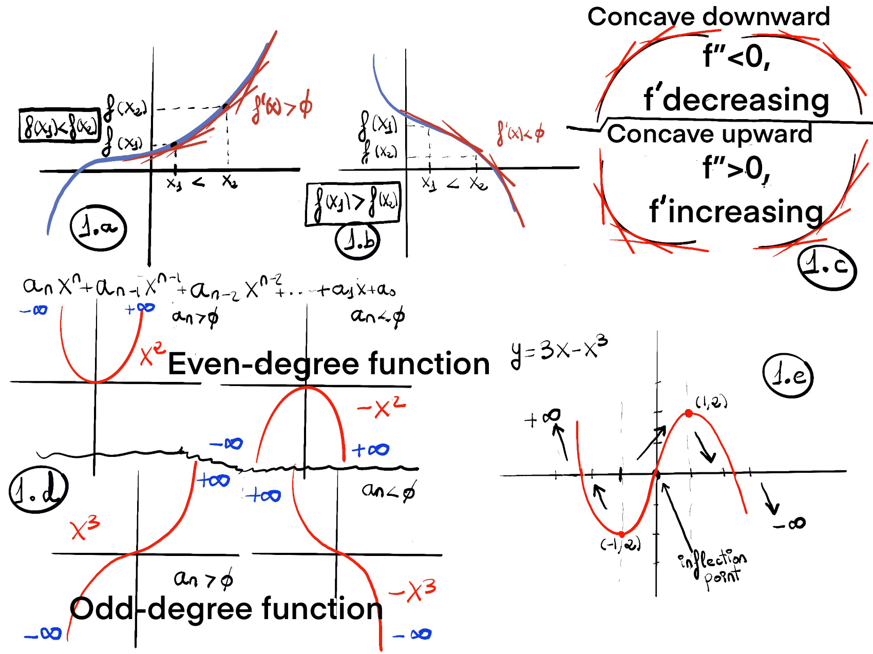
f is non-decreasing (increasing) on an interval I $\iff \forall a, b \in I, a \lt b \implies f(a) \le f(b)$. f is strictly increasing on an interval I $\iff \forall a, b \in I, a \lt b \implies f(a) \lt f(b)$ (figures 1.a., 1.b).

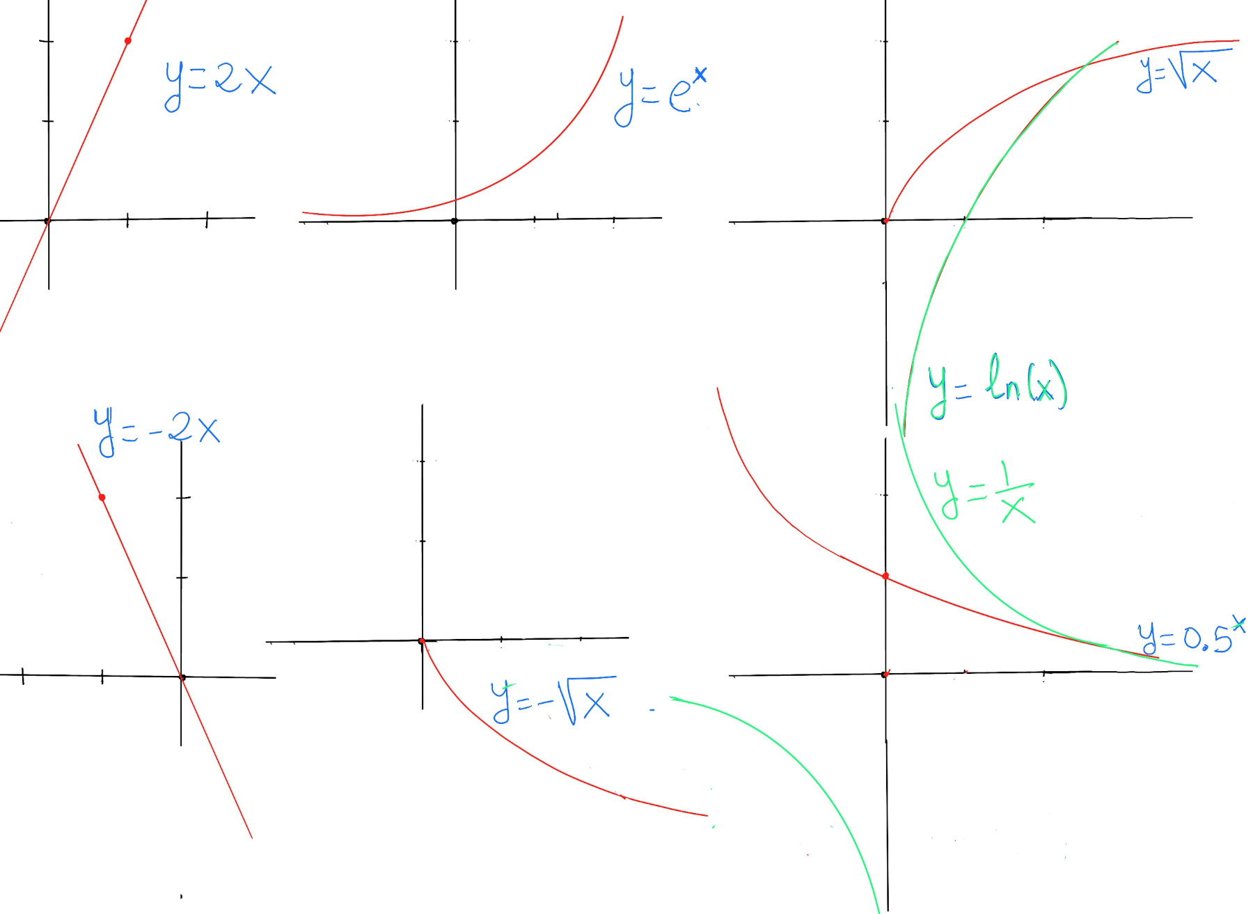
Strictly increasing functions: f(x) = 2x on ℝ; the exponential function f(x) = e^x on ℝ; the natural logarithm function f(x) = ln(x) on $(0, \infin)$; and the square root function f(x) = $\sqrt{x}$ on $[0, \infin)$.

f is non-increasing (decreasing) on an interval I $\iff \forall a, b \in I, a \lt b \implies f(a) \ge f(b)$. f is strictly decreasing on an interval I $\iff \forall a, b \in I, a \lt b \implies f(a) \gt f(b)$. f is contant on I $\iff \forall a, b \in I \implies f(a) = f(b)$.

Strictly decreasing functions: f(x) = -2x on ℝ; f(x) = $-\sqrt{x}$ on $[0, \infin)$; $f(x) = 2^{-x} = \left(\frac{1}{2}\right)^x = (0.5)^x$ on ℝ, this is classic example of exponential decay, that is, exponential functions with a base between 0 and 1 that is very common in physics (radioactive decay), finance (depreciation), and probability (geometric distributions); the reciprocal function f(x) = ¹⁄_x. f(x) = 3, f(x) = 7 are constant functions on any interval.  

Read left to right along the graph: if the graph never goes down it is non‑decreasing (it rises or stays flat); if it never goes up it is non‑increasing (it falls or stays flat); if it stays at the same height it is constant.

Derivative tests

The derivative of the function f(x) is used to determine whether a function is increasing, decreasing or constant on an interval.

Theorem. Derivative test for monotonicity. Let f be differentiable on an interval I. Then:

• If $f'(x) \ge 0$ for all $x \in I$, then f is non‑decreasing on I.

Take any two points a < b in I. By the Mean Value Theorem, there exists some $c\in (a, b)$ such that: $f'(c)=\frac{f(b)-f(a)}{b-a}.$ Since $f'(c) \geq 0$ and b -a > 0, it follows that $f(b)-f(a) \geq 0$. Thus, $f(b)\geq f(a)$, meaning f is non‑decreasing. The other cases follow similarly.

• If $f'(x) \gt 0$ for all $x \in I$, then f is strictly increasing on I.
• If $f'(x) \le 0$ for all $x \in I$, then f is non‑increasing on I.
• If $f'(x) \lt 0$ for all $x \in I$, then f is strictly decreasing on I.
• If f’(x) = 0 for all x on some interval I (∀x ∈ I), then f(x) is constant on I.

In other words, the intervals where a function is increasing (or decreasing) correspond to the intervals where its derivative is positive (or negative). The derivative f’(x) measures the instantaneous slope of the tangent line to the graph at x. A positive slope means the graph rises as x increases, a negative slope means it falls, and a slope of zero at a point means the tangent line is horizontal at that point; if f′(x)=0 for every x in an interval, then the graph is flat there and f is constant on that interval.

Definition. A critical point is a point in the domain of the function where the function is either not differentiable or the derivative is equal to zero. The value of the function at a critical point is called a critical value.

Critical points are the places where monotonicity can change. If f′ changes sign from positive to negative at a critical point then that point is a local maximum; if the sign changes from negative to positive it is a local minimum. If the sign does not change, then the critical point is neither a local maximum nor a local minimum. It could be a point of inflection (a point where the concavity changes; concave up f’’(x) > 0 switches to concave down f’’(x) < 0 or vice versa, e.g., f(x) = $x^3$, the critical point is at x = 0, the slope fattens, but the function keeps increasing, f’(x) = $3x^2 \ge 0, \forall x \in \mathbb{R}$) or a flat plateau (it occurs when the derivative is zero over an interval, not just at a single point, $f(x) = \begin{cases} 1, &0\leq x\leq 2 \\\\ x, &\mathrm{otherwise} \end{cases}$).

How to find increasing and decreasing intervals

1. Differentiate the function. This derivative tells us the slope of the tangent line at each point.
2. Identify Critical Points. Solve f’(x) = 0. As it was previously stated, a critical point is a point in the domain of the function where the function is either not differentiable or the derivative is equal to zero. In other words, these are points where the function’s behavior may change.
3. Partition the Domain. Use the critical points and any domain endpoints to divide the real line into intervals, e.g., if f critical points are x = -2 and 1, then we divide the real line into these intervals: $(-\infty ,-2),(-2,1),(1,\infty)$.
4. Analyze the sign of f’(x) on these intervals. Given an interval (a, c), pick a test point b in this interval, a < b < c. Calculate f’(b). If f’(b) is positive, then f(x) is increasing ↗ on that interval (a, c). If f’(b) is negative, f(x) is decreasing on ↘ that interval (a, c).

Solved examples

• A linear function is written as: y = mx + b, where m is the slope of the line and b is the y-intercept. f’(x) = m. The derivative is constant. No critical points exist (unless m=0, in which case the function is constant). The slope determines whether the linear function is increasing or decreasing. If the slope is positive (m > 0), the linear function (f'(x) > 0) is increasing ↗ on the entire domain. If the slope is negative (m < 0), the linear function (f'(x) < 0) is decreasing ↘ on the entire domain. If the slope is zero (m = 0), the linear function is a constant function, e.g., f(x) = 3x +5, f’(x) = 3 ⇒ f’(x) > 0 ⇒ f is increasing ↗.
• f(x) = (x -5)² (Figure i). f’(x) = 2·(x-5). Critical points: Solve f’(x) = 0 ⇒ 2(x-5) = 0 ↭ x = 5. Intervals:

1. x < 5, 2·(x-5) < 0 (or alternatively choose a point, e.g., x = 0, f’(0)=2·(-5)= -10) ⇒ f’(x) < 0 ⇒ f is decreasing ↘
2. x > 5, 2·(x-5) < 0 (or alternatively choose a point, e.g., x = 6, f’(6)=2·1= 2) ⇒ f’(x) > 0 ⇒ f is increasing ↗.
3. At x = 5, f(5) = 0. This is the minimum point since the parabola opens upward (a = 1 > 0).

• General Quadratic Function. The graph of a quadratic function ax² + bx + c is a parabola. It has an extreme point, called the vertex where the curve changes direction. Derivative: f’(x) = 2ax + b. Critical point (vertex): solve f’(x) = 0 $\implies x = \frac{-b}{2a}$. This is the axis of symmetry of the parabola.

1. If a > 0 (parabola opens upwards), the vertex represents the lowest point on the curve and its y-coordinate is the minimum value of the quadratic function. Domain(f) = ℝ, Range: y ≥ f($\frac{-b}{2a}$), f is decreasing to the left of x = $\frac{-b}{2a}$ (minimum) and increasing to the right of x = $\frac{-b}{2a}$.
2. If a < 0 (parabola opens downwards), the vertex represents the highest point on the curve, and its y-coordinate is the maximum value. Domain(f) = ℝ, Range: y ≤ f($\frac{-b}{2a}$), f is increasing to the left of x = $\frac{-b}{2a}$ (maximum) and decreasing to the right of x = $\frac{-b}{2a}$.

In either case, the vertex is a turning point on the graph. The graph is also symmetric with a vertical line drawn through the vertex, called the axis of symmetry $x = \frac{-b}{2a}$, So, the graph of the function is increasing on one side of the axis and decreasing on the other side.

• f(x) = $x·e^{-x}$ (Figure ii). Derivative: f’(x) = $e^{-x}-xe^{-x} = e^{-x}(1-x).$ Since $e^{-x}>0$ for all real x, the sign of f’(x) depends entirely on (1-x).

Critical points: f’(x) = 0 ⇒[The range of the exponential function is all positive real numbers] 1 -x = 0 ↭ So, the critical point is at x = 1. Behavior on Intervals:

1. x < 1, (1 -x) > 0 ⇒ f’(x) > 0 ⇒ f is increasing ↗.
2. x > 1, (1 -x) < 0 ⇒ f’(x) < 0 ⇒ f is decreasing ↘. Thus, the function increases until x = 1, then decreases afterward, so x = 1 is a local maximum and its maximum value is $\frac{1}{e}$.

• f(x) = x³ +3x² -9x +12 (Figure iii). Derivative: f’(x) = 3x² +6x -9 = 3·(x² +2x -3) = 3·(x +3)(x -1). Critical points: Solve f’(x) = 0 ⇒ 3·(x +3)(x -1) = 0 ↭ x = -3 or 1, and so there are three intervals to investigate:

1. $(-\infty ,-3)$: x < -3, e.g., x = -4, f’(-4) = 3·(-1)·(-5) = 15 > 0 ⇒ f’(x) > 0 ⇒ f is increasing ↗.
2. (-3, 1): -3 < x < 1, e.g., x = 0, f’(0) = 3·3·(-1) = -9 < 0 ⇒ f’(x) < 0 ⇒ f is decreasing ↘.
3. $(1,\infty )$: x > 1, e.g., x = 2, f’(2) = 3·5·1 = 15 > 0 ⇒ f’(x) > 0 ⇒ f is increasing ↗.

At x = -3: derivative changes from positive to negative, hence x = -3 is a local maximum. f(-3) = $(-3)^3+3(-3)^2-9(-3)+12=-27+27+27+12=39$, (-3, 39). At x = 1: derivative changes from negative to positive, hence x = 1 is a local minimum. $f(1)=1^3+3(1)^2-9(1)+12=1+3-9+12=7$, (1, 7).

• f(x) = 2x³ +3x² -36x (Figure iv).

1. Domain: All real numbers (ℝ). Since it’s a cubic polynomial with positive leading coefficient, the range is all real numbers: $\mathbb{R}$.
2. y-intercept: f(0) = 0, (0, 0). x-intercept: Solve f(x) = 0. $x(2x^2 + 3x - 36) = 0$. Then, x = 0 or $x = \frac{-3 \pm \sqrt{297}}{4} = \frac{-3 \pm 3\sqrt{33}}{4}$, (-5.058, 0) and (3.558, 0).
3. No symmetry (neither even nor odd).
4. No asymptotes. No vertical/horizontal/obliques asymptotes. Polynomials do not have horizontal or vertical asymptotes.
5. Critical points. f’(x) = 6x² + 6x -36 = 6(x² +x -6) = 6·(x+3)·(x-2). f’(x) = 0 ⇒ 6·(x+3)·(x-2) = 0 ↭ x = -3 and x = 2.
6. Sign analysis. x < -3, e.g., -4, f’(-4) = 6·(-1)·(-6) = 36 > 0 ⇒ f’(x) > 0 ⇒ f is increasing ↗. -3 < x < 2, e.g., 0, f’(0) = 6·3·(-2) < 0 ⇒ f’(x) < 0 ⇒ f is decreasing ↘. x > 2, e.g., 3, f’(3) = 6·6·1 > 0 ⇒ f’(x) > 0 ⇒ f is increasing ↗. Increasing on: $(-\infty, -3) \cup (2, \infty)$ and decreasing on: $(-3, 2)$.
7. Local maximum at x = -3: f(-3) = 2(-27) + 3(9) - 36(-3) = -54 + 27 + 108 = 81, (-3, 81). Local minimum at x = 2, f(2) = 2(8) + 3(4) - 36(2) = 16 + 12 - 72 = -44, (2, -44).
8. Concavity. f’’(x) = 12x + 6 = 6(2x + 1). Inflection point: f’’(x) = 0, then $x = -\frac{1}{2}$. If $x < -\frac{1}{2}: f''(x) < 0$, Concave down. If $x > -\frac{1}{2}: f''(x) > 0$, Concave up.
9. End Behaviour. As $x \to +\infty, f(x) \to +\infty$ (since leading term $2x^3$ dominates). As $ x \to -\infty, f(x) \to -\infty$.

• f(x) = 3x -x³ (Figure 1.e).

1. Domain: All real numbers $\mathbb{R}$ (polynomial). Since it’s a cubic polynomial with negative leading coefficient, the range is all real numbers, $\mathbb{R}$.
2. y-intercept: f(0) = 0, (0, 0). x-intercepts: Solve f(x) = 0: $3x - x^3 = x(3 - x^2) = 0$, then $(-\sqrt{3}, 0), (\sqrt{3}, 0)$.
3. Symmetry. Odd function (symmetric about the origin), $f(-x) = -3x + x^3 = -(3x - x^3) = -f(x)$.
4. Asymptotes. No asymptotes (polynomial).
5. f’(x) = 3 -3x² = 3(1-x²) = 3(1-x)(1+x). Critical points, f’(x) = 0, x = ±1, f(1)=2, f(-1-)=-2. Critical values: (−1, −2), (1, 2).
6. Sign analysis. x < -1, f’(-2) = 3 -3·4 = -9 < 0, f’(x) < 0 ⇒ f is decreasing ↘; -1 < x < 1, f’(0) = 3 -3·0 = 3 > 0, f’(x) > 0 ⇒ f is increasing ↗; x > 1, f’(2) = 3·-3·4 = -9 < 0, f’(x) < 0 ⇒ f is decreasing. Increasing on: (-1, 1), decreasing on: $(-\infty, -1) \cup (1, \infty)$.
7. Local minimum at x = -1: (-1, -2). Local maximum at x = 1: (1, 2).
8. f’’(x) = -6x. Inflection point: f’’(x) = 0, x = 0, (0, 0). x < 0: f’’(x) > 0, then f is concave up. x > 0: f’’(x) < 0, then f is concave down.
9. End Behaviour. As $x \to +\infty, f(x) \to -\infty$ (since $-x^3$ dominates). As $x \to -\infty, f(x) \to +\infty$
10. Graphs comes from $+\infty$ as $x \to -\infty$, passing through x-intercept $(-\sqrt{3}, 0)$ and decreasing to local minimum at (-1, -2). Then, it increases from (-1, -2) through inflection point at (0, 0) to local maximum at (1, 2). Finally, it decreases from (1, 2) through x-intercept at $(\sqrt{3}, 0)$ to $\infin$.

• $\frac{x + 1}{x + 2}$. The plot is shown in Figure 1.a.

1. Domain: $\mathbb{R} \setminus \{ -2 \}$.
2. x-intercept: Set numerator = 0, x = -1, (-1, 0). y-intercept: $f(0) = \frac{1}{2} = 0.5, (0, 0.5)$.
3. No symmetry (neither even nor odd).
4. Vertical Asymptote, x = 2, $\lim_{x \to -2^{-}} f(x) = +\infty, \lim_{x \to -2^{+}} f(x) = -\infty$. $\lim_{x \to \pm\infty} f(x) = \lim_{x \to \pm\infty} \frac{x+1}{x+2} = 1$, y = 1 is horizontal asymptote. $f(x) -1 = \frac{x+1-(x+2)}{x+2}= \frac{-1}{x+2}$. As $x \to -\infty, f(x) \to 1^{+}$ (from above). As $x \to +\infty, f(x) \to 1^{-}$ (from below).
5. f’(x) = $\frac{1}{(x+2)^2}$ > 0 ∀ x ∈ ℝ, x ≠ -2 ⇒ f is increasing (-∞, -2) and (-2, ∞). Critical points are those where the derivate is zero or the derivate is not defined, but x = -2 is not in the domain.
6. Concavity. $f''(x) = -\frac{2}{(x+2)^3}$. $x < -2: (x+2)^3 < 0 \implies f''(x) > 0$, f is concave up. $x > -2: (x+2)^3 > 0 \implies f''(x) < 0$, f is concave down. No inflection points (concavity changes at x = -2, but not in domain).
7. The graph consists of two disconnected branches. Left branch (x < −2): Lies entirely without crossing above y = 1, increases from y ≈ 1 to +∞, and concave up. Right branch (x > −2): Increases from -∞ to y ≈ 1, crosses the x-axis at (-1, 0) and the y-axis at (0, 0.5), and concave down.

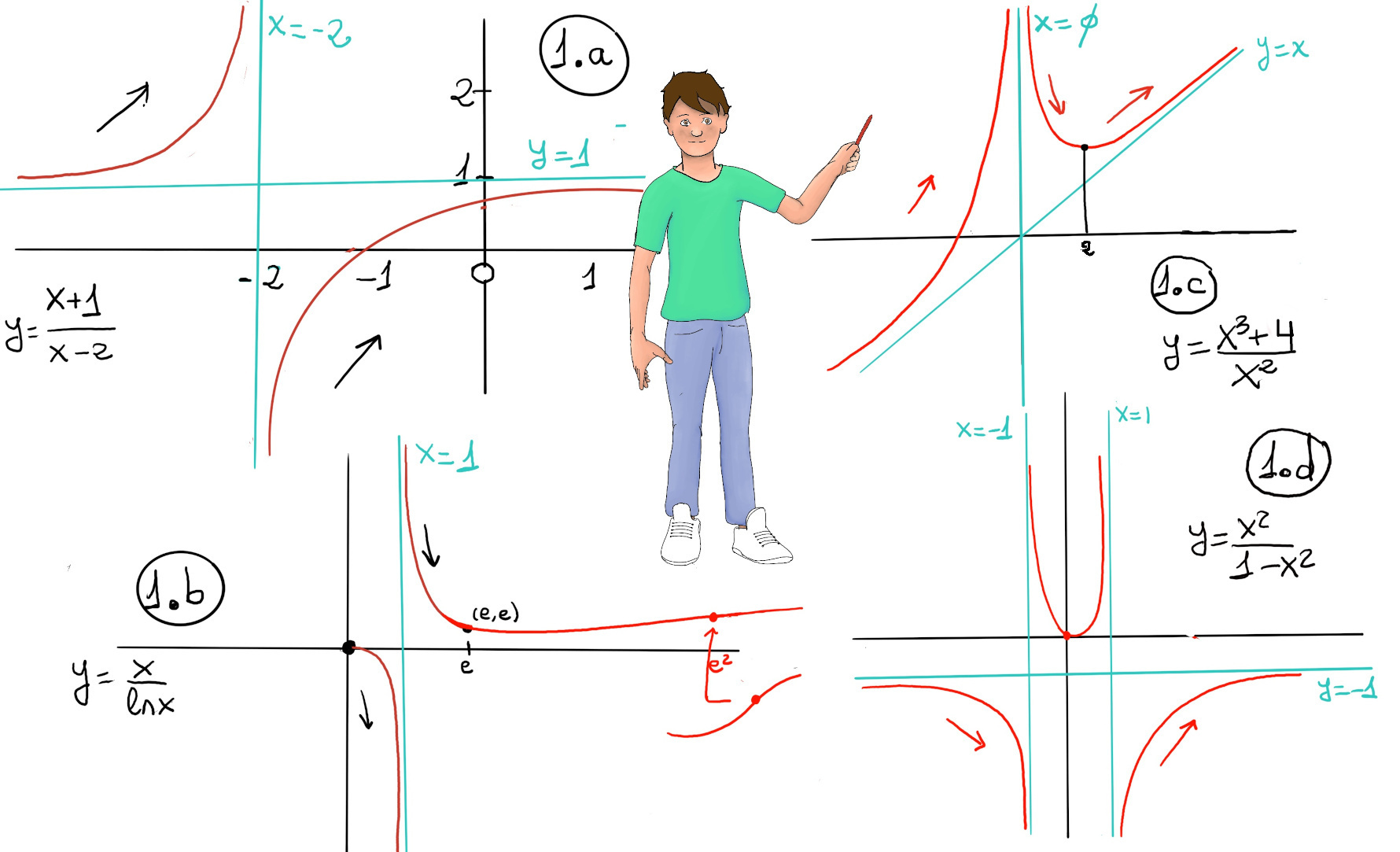
• $\frac{x^{3}+4}{x^{2}}$. The plot is shown in Figure 1.c.

1. Domain: $\mathbb{R} \setminus \{ 0\} = (-\infty, 0) \cup (0, \infty)$. For x < 0: f(x) increases continuously from $-\infty$ to $+\infty$, f covers all real numbers. Overall range: $\mathbb{R}$.
2. x-intercept: Solve $x^3 + 4 = 0 \implies x^3 = -4 \implies x = -\sqrt[3]{4}, (-\sqrt[3]{4}, 0).$ y-intercept: None (function undefined at x = 0).
3. No symmetry (neither even nor odd).
4. Vertical Asymptote at x = 0, $\lim_{x \to 0^-} f(x) = \lim_{x \to 0^+} f(x) = +\infty$, so the graph goes to positive infinity on both sides of the asymptote. Perform polynomial division: $(x) = \frac{x^3+4}{x^2} = x + \frac{4}{x^2}$. As $x \to \pm\infty, \frac{4}{x^2} \to 0, \text{ so } f(x) \to x$, y = x is an oblique asymptote. Since $\frac{4}{x^2} > 0, \forall x \neq 0, f(x) > x \forall x \neq 0$.
5. f’(x) = $\frac{3x^{4}-(x^{3}+4)2x}{x^{4}}= \frac{3x^{4}-2x^{4}-8x}{x^{4}}= \frac{x^{3}-8}{x^{3}} = 1 - \frac{8}{x^3}$. f’(x) = 0 ⇒ x = 2. Critical points: 0, 2.
6. Sign analysis: x < 0, f’(x) > 0 ⇒ f increasing ↗. 0 < x < 2, f’(x) < 0 ⇒ f decreasing ↘. x > 2, f’(x) > 0 ⇒ f increasing ↗. Increasing on: $( (-\infty, 0) \cup (2, \infty)$. Decreasing on: $(0, 2)$.
7. Local minimum at (2, 3). No local maximum, function increases to $+\infty$ near zero.
8. $f''(x) = \frac{24}{x^4}. f''(x) > 0 \forall x \neq 0$. Concave up on: $(-\infty, 0) \text{ and } (0, \infty)$. No inflection points (concavity doesn’t change).
9. The graph has two disconnected branches. Left branch x < 0: it increases from $-\infty$ (always above the line y = x, but without touching it) to $+\infty$, crosses the x-axis at $x = -\sqrt[3]{4}$, and is always concave up. Right branch x > 0: it decreases from $+\infty$ to the local minimum at (2, 3), then increases to $+\infty$ (always above the line y = x, but without touching it), and is always concave up.

Bibliography

1. NPTEL-NOC IITM, Introduction to Galois Theory.
2. Algebra, Second Edition, by Michael Artin.
3. LibreTexts, Calculus. Abstract and Geometric Algebra, Abstract Algebra: Theory and Applications (Judson).
4. Field and Galois Theory, by Patrick Morandi. Springer.
5. Michael Penn, Andrew Misseldine, blackpenredpen, and MathMajor, YouTube’s channels.
6. Contemporary Abstract Algebra, Joseph, A. Gallian.
7. MIT OpenCourseWare, 18.01 Single Variable Calculus, Fall 2007 and 18.02 Multivariable Calculus, Fall 2007, YouTube.
8. Calculus Early Transcendentals: Differential & Multi-Variable Calculus for Social Sciences.