Local Extrema. First and Second Derivative Tests

The problem is not the problem. The problem is your attitude about the problem, Captain Jack Sparrow

Recall

Definition. A function f is a rule, relationship, or correspondence that assigns to each element x in a set D, x ∈ D (called the domain) exactly one element y in a set E, y ∈ E (called the codomain or range).

• The pair (x, y) is denoted as y = f(x) where: x is the independent variable (input) and y is the dependent variable (output). Often, both the domain D and codomain E are the set of real numbers ℝ or subsets of ℝ.

• D is the domain, the set of all possible inputs. E is the codomain or range, the set of all possible outputs.

• Key property💡: Each input has exactly one output. (No input is assigned two different outputs — this is the vertical line test!)

• Examples: constant, f(x) = c, horizontal line, slope = 0; linear, f(x) = mx + b, straight line, constant slope m and y-intercept b; quadratic $f(x) = ax^2 + bx + c$, u-shaped or inverted U, opens up (a > 0) or down (a < 0), vertex at x = $\frac{-b}{2a}$, symmetry about vertical axis through vertex; polynomial, $f(x) = a_n x^n + \dots + a_0$, a smooth and continuous curve, n roots (counting multiplicity), end behaviour determined by its leading term $a_n x^n$; exponential function, $f(x) = a \cdot b^x, a \ne 0, b \gt 0$, rapid growth (b > 1) or decay (0 < b < 1); trigonometric functions, $\sin(x), \cos(x), \tan (z)$ oscillatory, periodic behavior (period 2π for sin/cos, π for tan), sin and cos are bounded between -1 and 1, but tan is unbounded; step function $f(x) = \lfloor x \rfloor$, greatest integer ≤ x, constant on intervals [n, n+1), jumps at integers, its graph is a staircase shape; absolute value f(x) = |x|, V-shaped graph, slope changes at 0.

• Functions can be expressed in multiple forms, each useful in different contexts: verbal description, table of values (list of pairs), algebraic formula, graph, piecewise definition, recursive definition, parametric or integral form, and series representation.

• Evaluating a function means finding or computing the output value f(x) for a given input value x. f(x) = $x^2-2x +4, f(2) = 2^2 -2\cdot 2 + 4 = 4 - 4 + 4 = 4, f(0) = 0^2 -2\cdot 0 + 4 = 4, f(1) = 1^2 -2\cdot 1 + 4 = 1 -2 +4 = 3$

• The x-intercept is any point on the graph that intersects or crosses the x-axis. In other words, it is the value of x when the function (y-coordinate or y-value) is zero. The y-intercept is the point where the graph intersects or crosses the y-axis. y-coordinate of the point whose x-coordinate is 0, e.g., 2x - 3y = 6. x-intercept: set y = 0 → 2x = 6 ⇒ x=3, so (3, 0). y-intercept: set x = 0 → −3y = 6 ⇒ y = −2, so (0, −2).

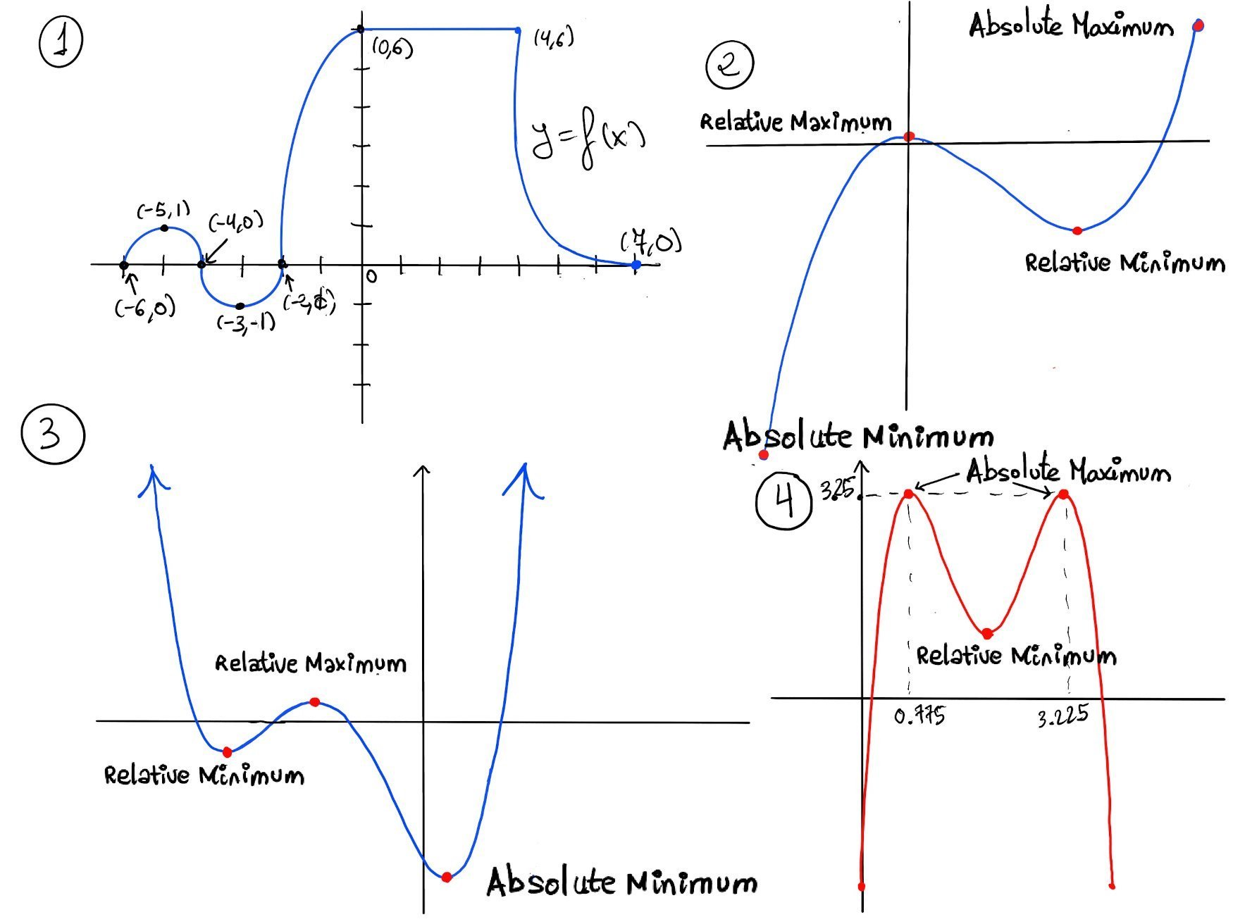
• f is said to have a local or relative maximum at c if there exists an interval (a, b) containing c ($c \in (a, b)$) such that f(c) ≥ f(x) $∀ x \in (a, b) ∩ D$. f is said to have a local or relative minimum at c if there exists an interval (a, b) containing c ($c \in (a, b)$) such that f(c) ≤ f(x) $∀ x \in (a, b) ∩ D$.💡Local extrema can only occur where the function stops rising or falling —either because the derivative is zero, the derivative doesn't exist, or you're at the edge of the domain.

First Derivative Test

First Derivative Test. It connects local extrema with changes in the sign of the derivative.

• If the derivate f’(x) changes sign from positive to negative (as we look from left to right at the graph) at a critical point x = c, then f(c) is a local maximum (a peak).
• If the derivate f′(x) changes sign from negative to positive at a critical point x = c, then f(c) is a local minimum (a valley).  

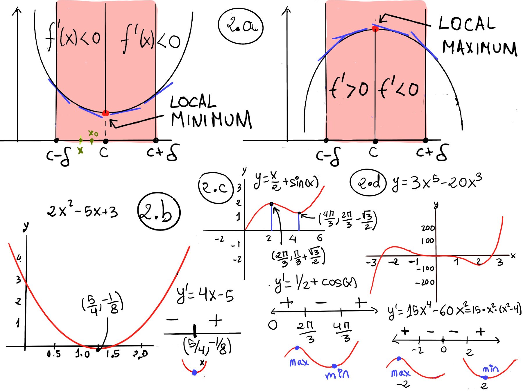
First Derivative Test. Let f be differentiable on an open interval containing c, except possibly at c itself, and let c be a critical point (so f′(c) = 0 or f′ is undefined). Then:

1. If f′(x) > 0 for x just to the left of c and f′(x) < 0 for x just to the right of c, then f(c) is a local maximum.
2. If f′(x) < 0 for x just to the left of c and f′(x) > 0 for x just to the right of c, then f(c) is a local minimum.
3. If f′(x) does not change sign at c (stays positive or stays negative), then f(c) is not a local extremum.

Proof.

Let’s confine ourself to the case of the minimum, the other case is completely analogous.

Assume that f is continuous on an interval containing c, differentiable on that interval except maybe at c. Hence, for some δ > 0: ∀x ∈ (c -δ, c), f’(x) < 0, ∀x ∈ (c, c + δ), f’(x) > 0.

Claim: f(c) is a local minimum, i.e. that for x close to c, f(x) ≥ f(c).

Lagrange’s Mean Value Theorem (LMVT) states that if a function is continuous on a closed interval [a, b] and differentiable on the open interval (a, b), then there exists at least one point $c \in (a, b)$ where the instantaneous rate of change (derivative) equals the average rate of change over the interval, $f'(c)=\frac{f(b)-f(a)}{b-a}$. In other words, the slope of the tangent at c equals the slope of the secant line joining (a, f(a)) and (b, f(b)).

Left side of c. Take any x with $ x\in (c-\delta, c)$. Consider the interval [x, c]. Since f is continuous on [x, c] and differentiable on (x, c), by MVT there exists $\xi \in (x, c)$ such that $f(c) - f(x) = f'(\xi)[c-x] \lt 0$ because c -x > 0 and $\xi \in (x, c) \subset (c-\delta, c) \leadsto f'(\xi) < 0.$ So for x to the left of c, f(x) > f(c).

Right side of c. Now take any $x \in (c, c +\delta)$. Consider the interval [c, x]. Again, MVT gives some $\eta\in (c,x)$ such that $f(x) - f(c) = f'(\eta)[x-c] \gt 0$ because x - c > 0 and $\eta \in (c, x)\subset (c, c + \delta) \leadsto f'(\eta) >0.$ So for x to the right of c, f(x) > f(c) as well.

Combining both sides: for all $x \neq c$ in a small enough neighborhood (sufficient close) to c we have f(x) > f(c). Therefore, f(c) is indeed a local minimum.

Second Derivative Test

The Second Derivative Test is a convenient way to classify critical points algebraically, using information about concavity.

Second Derivative Test. If the first derivate of a function at a point c is zero (f'(c) = 0) and the second derivate at this point exists, then: (i) If f''(c) > 0, then f(c) is a local minimum. (ii) If f''(c) < 0, then f(c) is a local maximum. (iii) If f''(c) = 0, the test is inconclusive.

f′′(c) > 0 ⇒ the graph is concave up near c (like a bowl), so a flat tangent there must be at the bottom → local minimum. f′′(c) < 0 ⇒ concave down near c (like an upside-down bowl), so a flat tangent is at the top → local maximum.

Proof.

Let’s again consider only the local minimum case.

Assume f′(c) = 0, f′′(c) > 0, and f′′ is continuous near c. Since f’’(c) > 0, and f′′ is continuous near c, ∃δ > 0: ∀x ∈ (c - δ, c + δ), f′′(x) > 0.

So, the first derivate f’ is increasing on (c - δ, c + δ). Because f′(c) = 0 and f’ is increasing:

• For x < c but close to c, we must have f’(x) < 0
• For x > c but close to c, we must have f’(x) > 0

This is exactly the sign change pattern of the First Derivative Test for a local minimum. So f(c) is a local minimum. The case f’’(c) < 0 is analogous and gives a local maximum. If f’’(c) = 0, the second derivative test tells us nothing: the point could be a local extremum, an inflection point, or something more exotic.

Examples

• Quadratic function. Find local extrema for y = 2x² -5x + 3 (Figure 2.b).

1. Compute the derivative: y’ = 4x -5.
2. Find critical points by solving y′ = 0: 0 = 4x -5, x = ⁵⁄₄. This is the only critical point.
3. Second derivative: y’’= 4 > 0, the parabola is concave up, so by the Second Derivative Test, f(⁵⁄₄) is a local minimum and the minimal value is $f\Bigl(\frac{5}{4}\Bigr) = 2\Bigl(\frac{5}{4}\Bigr)^2 - 5\Bigl(\frac{5}{4}\Bigr) + 3 = 2 \cdot \frac{25}{16} - \frac{25}{4} + 3 = \frac{50}{16} - \frac{100}{16} + \frac{48}{16} = \frac{50 - 100 + 48}{16} = \frac{-2}{16} = -\frac{1}{8}.$
4. For a quadratic opening upwards (with positive leading coefficient$x^2$, 1 > 0), this local minimum is also the global minimum (the lowest value of the function on $\mathbb{R}$).
5. Vertex (minimum point): $\left(\frac{5}{4}, -\frac{1}{8} \right)$. You can also quickly recall the vertex formula for any quadratic $ax^2 + bx + c$: $x_{\text{vertex}} = -\frac{b}{2a} = -\frac{-5}{2\cdot2} = \frac{5}{4}$.
6. No maximum, the function goes to $+∞$ as $x \to \pm ∞$.

• Calculate local maximum and minimum points for y = ¹⁄₂x + sin(x) on [0, 2π] (Figure 2.c).

1. Compute derivative: y’ = ¹⁄₂ + cos(x).
2. Find critical points by solving y’ = 0 ⇒ cos(x) = -¹⁄₂. On [0, 2π], this happens at x = ^2π⁄₃, x = ^4π⁄₃.
3. We classify these critical points using the First or Second Derivative Test. y′′ = −sin(x). At $x = \frac{2\pi}{3}, \sin\left(\frac{2\pi}{3}\right) = \frac{\sqrt{3}}{2} > 0$, so $y''\Bigl(\frac{2\pi}{3}\Bigr) = -\frac{\sqrt{3}}{2} < 0,$ local maximum. At $x = \frac{4\pi}{3}, \sin\left(\frac{4\pi}{3}\right) = -\frac{\sqrt{3}}{2}$, so $y''\Bigl(\frac{4\pi}{3}\Bigr) = +\frac{\sqrt{3}}{2} > 0,$ local minimum.
4. So on $[0, 2\pi]$, the function has a local maximum at ($\frac{2π}{3}, \frac{π}{3}+\frac{\sqrt{3}}{2}$) and a local minimum at ($\frac{4π}{3}, \frac{2π}{3}-\frac{\sqrt{3}}{2}$).

• Calculate local maximum and minimum points for the quintic polynomial y = 3x⁵ -20x³ (Figure 2.d).

1. Let’s find the critical points by setting the derivate y’ = 15x⁴ -60x² to zero. 15x⁴ -60x² = 0 ↭ 15x²(x²-4) = 0. So, the critical points are x = 0, x = 2, and x = -2.
2. Use the second derivative test to determine the nature of each critical point and calculate local maximum and minimum points. y’’ = 60x³ -120x. y’’(0) = 0, y’’(2) > 0, and y’’(-2) < 0.

Therefore, it has a local minimum at x = 2 and a local maximum at x = -2. The critical point x = 0 is not a local extremum; it’s a point of inflection.

In the previous example (Figure 1), f has local or relative minimum points at -6, -3, and 7, and local or relative maximum points at -5, 0, and 4. On the open interval (0, 4), the function is constant, and therefore every point is both a local or relative maximum and minimum point. Futhermore, (-4, 0), (-2, 0), (0, 6), and (4, 6) are points of inflection.

Bibliography

1. NPTEL-NOC IITM, Introduction to Galois Theory.
2. Algebra, Second Edition, by Michael Artin.
3. LibreTexts, Calculus. Abstract and Geometric Algebra, Abstract Algebra: Theory and Applications (Judson).
4. Field and Galois Theory, by Patrick Morandi. Springer.
5. Michael Penn, and MathMajor.
6. Contemporary Abstract Algebra, Joseph, A. Gallian.
7. YouTube’s Andrew Misseldine: Calculus. College Algebra and Abstract Algebra.
8. MIT OpenCourseWare 18.01 Single Variable Calculus, Fall 2007 and 18.02 Multivariable Calculus, Fall 2007.
9. Calculus Early Transcendentals: Differential & Multi-Variable Calculus for Social Sciences.