Derivate and Tangent Lines

If you wish to make an apple pie from scratch, you must first invent the universe, Carl Sagan

Tangent Line: Geometric Meaning

Definition. Let y = f(x) be a function. The tangent line to the graph of f at a point P = (x₀, y₀) = (x₀, f(x₀)) is the straight line that just touches the curve at that particular point and -1.a.-, shares the curve's slope there. Intuitively, the tangent line is the best linear approximation to the curve near the point of contact P.

The equation of the tangent line at P = (x₀, y₀) is y - y₀ = m (x - x₀), where y₀ = f(x₀) and m is the slope of the tangent line. The slope of the tangent line at a point P(x₀, y₀) is the derivative of the function f at that point, m = f’(x₀). In other words, the derivative of a function at a point f’(x₀) measures the slope of the tangent line to the graph at that point.  

From Secant Lines to the Tangent Line

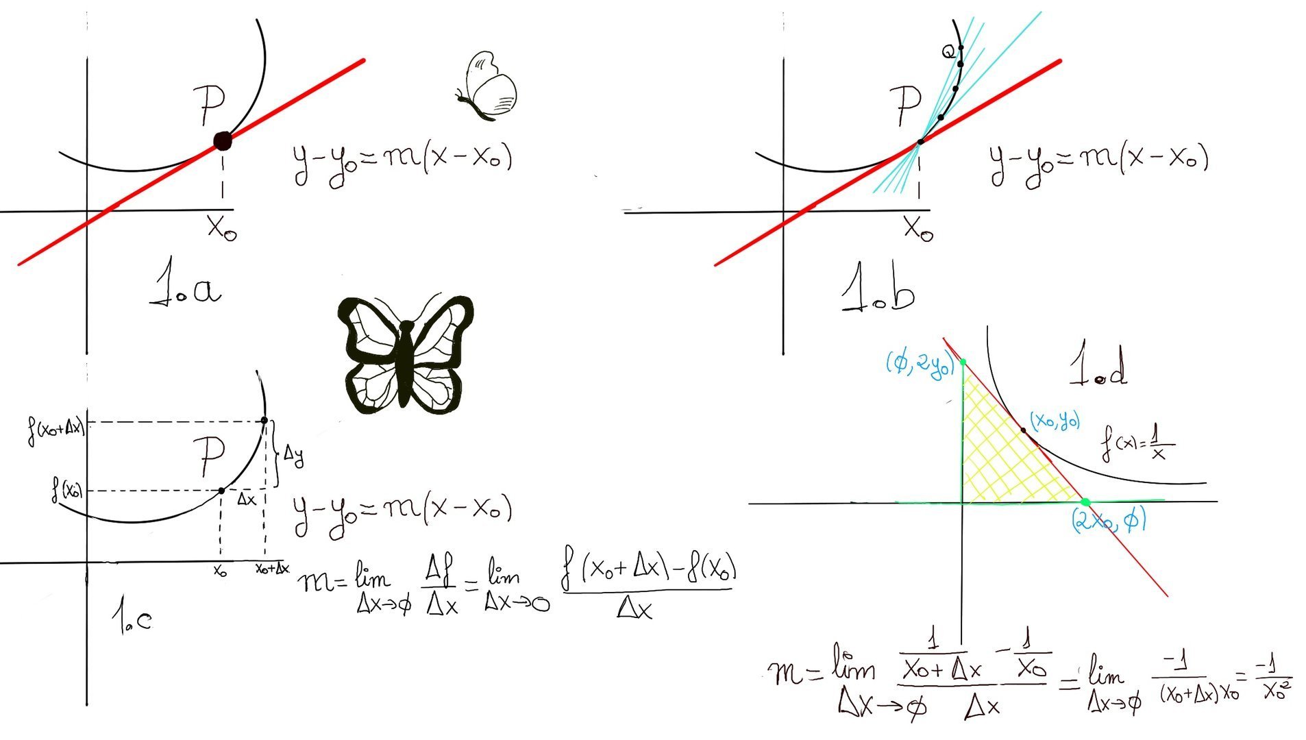
To understand where the derivative comes from, consider two points on the curve: P = $(x_0, f(x_0))$ (P is obviously fixed) and Q = $(x_0 + \Delta x, f((x_0 + \Delta x)))$. The line passing through P and Q is called a secant line. Its slope is $\frac{\Delta f}{\Delta x} = \frac{f((x_0 + \Delta x))-f(x_0)}{\Delta x}$

As the point Q moves closer to P (that is, as $\Delta x \to 0$), the secant line approaches the tangent line. The derivative is the limit of the slopes of secant lines as they approach the tangent line (1.b., 1.c.). Formally, m = f’(x₀) = $\lim_{\Delta x \to 0} \frac{\Delta f}{\Delta x}$ = $\lim_{\Delta x \to 0} \frac{f(x_0+\Delta x) -f(x_0)}{\Delta x}$

Physical interpretation: Velocity

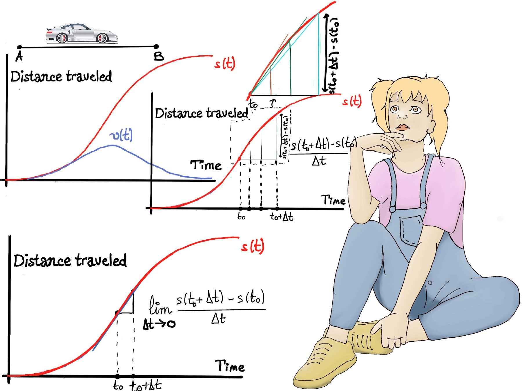
Let’s imagine a car 🚗 traveling from Madrid to Barcelona. We could graph this motion (s(t)), letting the vertical axis (y) represents the distance traveled by the vehicle at time t (measured in units such as meters, kilometers, miles, etc.), and the horizontal axis (t) represents the time taken to travel the distance (measured in units such as seconds, minutes, hours, etc.).

At the beginning, the curve is quite shallow (commercial cars accelerate slowly), then for the next seconds, as the car speeds up, the distance traveled in a given time get larger so the curve become steeper. Near the destination, the car slows down again, and the curve flattens. We can also plot velocity.

The average velocity over a time interval $[t_0, t_0 + \Delta t]$ can be thought of as the average of all speedometer readings and is often calculated using the following formula $\frac{distance~ traveled}{time~ of~ travel}$; more formally, $\frac{s(t_0 + \Delta t)-s(t_0)}{\Delta t}$.

Velocity is the rate of change of an object displacement or position with respect to time. Instantaneous velocity is the velocity of an object in motion at a specific point in time. It is the limit of these averages as the time interval shrinks (approaches zero), $v(t_0) = \lim_{\Delta t \to 0} \frac{s(t_0 + \Delta t)-s(t_0)}{\Delta t}$ (Figure below). Geometrically, instantaneous velocity is the slope of the tangent line to the distance traveled or position versus time graph at that instant.  

Example: f(x) = ¹⁄_x

We compute the derivative using the definition (Figure 1.d). Difference quotient, $\frac{f(x_0+\Delta x) -f(x_0)}{\Delta x} = \frac{\frac{1}{x_0+\Delta x} -\frac{1}{x_0}}{\Delta x} =[\text{Combine the fractions:}] \frac{1}{\Delta x} \frac{x_0-x_0-\Delta x}{(x_0+\Delta x)x_0} = \frac{1}{\Delta x} \frac{-\Delta x}{(x_0+\Delta x)x_0} = \frac{-1}{(x_0+\Delta x)x_0}$

 

Next, we take the limit: $\lim_{\Delta x \to 0} \frac{f(x_0+\Delta x) -f(x_0)}{\Delta x} = \lim_{\Delta x \to 0}\frac{-1}{(x_0+\Delta x)x_0} = \frac{-1}{x_0^{2}}$. So, $\boxed{f'(x)} = \frac{-1}{x^{2}}$

Observe that the slope is negative and as $x \to \infty$, the line tangent line become flatter (it has less and less slope).

Geometry of the Tangent Line to $y = \frac{1}{x}$

The tangent line at $(x_0, y_0)$, where $y_0 = \frac{1}{x_0}$ is y - y₀ = f’(x₀)(x - x₀) ↭ y - y₀ = ^-1⁄_x0² (x - x₀).

The x-intercept is the point where the tangent line crosses the x-axis, meaning the y-coordinate is always zero at that point. Set y = 0.

y - y₀ = 0 - y₀ = 0 - ¹⁄_x0 = ^-1⁄_x0² (x - x₀) = ^-x⁄_x0²+¹⁄_x0 ⇨ $\frac{x}{x_0^{2}}=\frac{2}{x_0}$ ⇨[Solving] x = 2x₀. The x-intercept is (2x₀, 0).

The y-intercept is the point where the tangent line crosses the y-axis, that is, x = 0. Because of symmetry (y = ¹⁄_x ↔ xy = 1 ↔ x = ¹⁄_y), the y-intercept is (0, 2y₀).

This symmetry reflects the fact that $y = \frac{1}{x}$ is invariant under swapping x and y.

Area of the Triangle Formed with the Axes

Let’s calculate or compute the area of triangles enclosed by the axes and the tangent line to y = ¹⁄_x. The area of a triangle is defined as the region enclosed by it three sides. It is equal to half of the base times height, i.e., A = ¹⁄₂base * height = ¹⁄₂(2x₀)(2y₀) =[y₀ = ¹⁄_x0] 2. Remarkably, the area is constant and does not depend on the point of tangency.

Alternative Definition of the Derivative

For convenience, instead of writing x₀, we usually fix x and let the increment vary. Writing h instead of $\Delta x$, we obtain the most standard and widely used definition of derivate. The derivative of f at x is defined as f'(x) = $\lim_{h \to 0} \frac{f(x+h) -f(x)}{h}.$

Differential

The term differential is used in calculus to refer to an infinitesimal change, that is, an infinitely small variation, difference, or change in some varying quantity or variable that depends on another. Differentials provide a powerful language for describing how small changes in one variable influence small changes in another.

Differentials allow us to relate infinitesimally small changes of variables through derivatives.

From Finite Changes to Infinitesimals

If x is a variable, a finite change in its value is often denoted by $\Delta x$. The corresponding finite change in a function y = f(x) is $\Delta y = f(x + \Delta x) - f(x)$.

The differential dx, by contrast, represents an infinitely small change in the variable x —a change so small that it captures only the local behavior of the function. While Δx is a finite increment, dx is conceptualized as an infinitesimal one.

Historical interpretation: Ratios of Infinitesimals

Historically, the derivative was thought of as a ratio of infinitesimal quantities: $\frac{dy}{dx}$ where dy is an infinitesimal change in y and dx is an infinitesimal change in x. This interpretation is based on the idea that if dx is an infinitesimally small change in x, then the corresponding change in y, denoted as dy, can be approximated by the tangent line, so dy is approximated by the derivative times dx: dy ≈ f'(x)dx or equivalently $\frac{dy}{dx} = f'(x)$. This approximation becomes exact in the limit as $dx \to 0$.

Geometrically, this means that for very small values of dx, the graph of f is almost indistinguishable from its tangent line. The differential dy measures the change along this tangent line rather than along the curve itself.

In motion, dx may represent an infinitesimal change in time, dy may represent an infinitesimal change in position, and $\frac{dy}{dx}$ corresponds to instantaneous velocity.

It is important to distinguish between:

• $\Delta y = f(x + \Delta x) - f(x)$ is the actual change in y (along the curve),
• $dy = f'(x)dx$ is the linear approximation to that change along the tangent line.

As $\Delta x \to 0$, the difference between Δy and dy becomes negligible.

Conclusion

The derivative of a function at a given input value, when it exists, is the slope of the tangent line to the graph of the function at that point and the instantaneous rate of change of the dependent variable with respect to the independent variable. It measures how one quantity responds locally to changes in another.

Formal Definition. A function f(x) is said to be differentiable at a point “a” in its domain, if its domain contains an open interval around “a”, and the limit $\lim _{h \to 0}{\frac {f(a+h)-f(a)}{h}}$ exists. In that case, the derivative of f at a is defined by f’(a) = L = $\lim _{h \to 0}{\frac {f(a+h)-f(a)}{h}}$.

More rigorously, f is differentiable at a if and only if for every positive real number ε, there exists a positive real number δ, such that for every h satisfying 0 < |h| < δ, we have $|\frac {f(a+h)-f(a)}{h} - L| \lt \epsilon$.

Examples

• Let’s calculate f’(x) where f(x) = $\sqrt{x}$

We begin with the definition:

$$ \begin{aligned} f'(x) &=\lim_{\Delta x \to 0} \frac{f(x+\Delta x) -f(x)}{\Delta x} \\[2pt] &[\text{Substituting } f(x)=\sqrt{x}]\\[2pt] &=\lim_{\Delta x \to 0} \frac{\sqrt{x+\Delta x} -\sqrt{x}}{\Delta x} \\[2pt] &[\text{This expression leads to an indeterminate form 0/0. To resolve it, we rationalize the numerator by multiplying and dividing by the conjugate.}] \\[2pt] &= \lim_{\Delta x \to 0} \frac{\sqrt{x+\Delta x} -\sqrt{x}}{\Delta x} \frac{\sqrt{x+\Delta x} +\sqrt{x}}{\sqrt{x+\Delta x} +\sqrt{x}} \\[2pt] &= \lim_{\Delta x \to 0} \frac{x+\Delta x-x}{\Delta x(\sqrt{x+\Delta x} +\sqrt{x})} \\[2pt] &=\lim_{\Delta x \to 0} \frac{\Delta x}{\Delta x(\sqrt{x+\Delta x} +\sqrt{x})} \\[2pt] &[\text{Cancelling } \Delta x, \Delta x \ne 0] \\[2pt] &=\lim_{\Delta x \to 0} \frac{1}{\sqrt{x+\Delta x} +\sqrt{x}} = \frac{1}{2\sqrt{x}} \end{aligned} $$

Thus, the derivative of $\sqrt{x}$ is $f'(x) = \frac{1}{2\sqrt{x}}$.

• Compute f’(0) where f(x) = |x| at x = 0. We now examine a function that is not differentiable at a point.

Using the definition, $f'(0) = \lim_{\Delta x \to 0} \frac{f(0+\Delta x) -f(0)}{\Delta x} = \lim_{\Delta x \to 0} \frac{|0+\Delta x| -|0|}{\Delta x} = \lim_{\Delta x \to 0} \frac{|\Delta x|}{\Delta x}$

We analyze the one-sided limits: $\lim_{\Delta x \to 0⁺} \frac{|\Delta x|}{\Delta x} = \lim_{\Delta x \to 0⁺} \frac{\Delta x}{\Delta x} = 1. \lim_{\Delta x \to 0⁻} \frac{|\Delta x|}{\Delta x} = \lim_{\Delta x \to 0⁻} \frac{-\Delta x}{\Delta x} = -1,$ the two one-sided limits are different, and so the limit does not exist. Therefore, f′(0) does not exist: the function ∣x∣ is not differentiable at x = 0. Geometrically, this corresponds to a sharp corner (cusp) at the origin.

• Find the equation of the tangent line to the function y = f(x) = x³ +4x -6 at the point x = 2.

Compute the point of tangency. f(2) = 2³ +4·2 -6 = 8 +8 -6 = 10. Thus, the point (2, 10).

Compute the derivative at x = 2. $\lim_{h \to 0} \frac{f(2+h)-f(2)}{h} = \lim_{h \to 0} \frac{(2+h)^3+4(2+h)-6-(2^3+4·2-6)}{h}$ [(a+b)³ = a³ +3a²b +3ab² +b²] $\lim_{h \to 0} \frac{h^3+2^3+3·4·h+3·2·h^2+8+4h-6-10}{h} = \lim_{h \to 0} \frac{h^3+6h^2+16h}{h} = \lim_{h \to 0} h^2+6h+16 = 16$ ⇒ The slope of the tangent line at 2 is f’(2) = 16.

Recall that the point-slope form of the equation of a line is given by: y - y₀ = m(x - x₀) where (x₀, y₀) is a point on the line and m (f’(x₀)) is the slope of the line at that point.

In our case with (x₀, y₀) = (2, 10) and m = 16, we get: y - 10 = 16(x -2) ⇒ The equation of the tangent line is y = 16x -32 +10 = 16x -22 $\implies \boxed{y = 16x -22}$

• Let’s calculate f’(x) where f(x) = xⁿ, n ≥ 1.

Using the definition: $\frac{f(x+\Delta x) -f(x)}{\Delta x} = \frac{(x+\Delta x)^{n} -x^{n}}{\Delta x} =[\text{Applying the binomial expansion:}] \frac{x^{n}+n\Delta xx^{n-1} + O((\Delta x)^{2}) -x^{n}}{\Delta x} = nx^{n-1} + O(\Delta x)$

$f'(x^{n})=\lim_{\Delta x \to 0}nx^{n-1} + O(\Delta x) = nx^{n-1}$. Thus, $\boxed{f'(x) = nx^{n-1}}$. This is the Power Rule, one of the foundational differentiation rules.

Average versus Instantaneous Rate of Change

If y is a function of x, y = f(x), a change in x from x₁ to x₂ is denoted by $\Delta x = x_2 - x_1$, and the corresponding change in y is denoted by $\Delta y = f(x_2) - f(x_1)$. The difference quotient $\frac{\Delta y}{\Delta x} = \frac{f(x_2) - f(x_1)}{x_2 - x_1}$ is called the average rate of change of y with respect to x. This is the slope of the line segment (secant line between P and Q) PQ, where P = P(x₁, f(x₁)) and Q = Q(x₂, f(x₂)).

The instantaneous rate of change of y with respect to x is the limit of the slopes of line segments PQ as Q gets closer and closer to P (the secant line approaches the tangent line as $x_2 \to x_1$), that is, $lim_{\Delta x \to 0}\frac{\Delta y}{\Delta x} = lim_{x_2 \to x_1}\frac{f(x_2) - f(x_1)}{x_2 - x_1} = f'(x_1).$

Therefore, the derivate f'(a) is the instantaneous rate of change of y = f(x) with respect to x when x = a.

Examples from Physics

• In physics, electrical current is defined as the rate at which electric charge flows through a conductor. The instantaneous electrical current is the derivate of charge with respect to time, $I = lim_{\Delta t \to 0}\frac{\Delta q}{\Delta t} = \frac{dq}{dt}$
• Speed is the rate of change of distance with time. Instantaneous speed is the limit of average speed as the time interval approaches zero or, alternatively, the derivate of distance with respect to time, that is, $v = lim_{\Delta t \to 0}\frac{\Delta s}{\Delta t} = \frac{ds}{dt}$

Example: If the distance that a person covers given at a certain time is d(t)=t² -t +2. Find the average speed for the first five seconds and the instantaneous speed after two seconds.

$v_m = \frac{d(t=5) - d(t=0)}{5} = \frac{(22 - 2)m}{5s} = 4 m/s.$

$v = lim_{\Delta t \to 0}\frac{\Delta s}{\Delta t} = \frac{ds}{dt} = 2t - 1, v(2) = d'(2)= 2·3-1 = 3 m/s.$

Bibliography

1. NPTEL-NOC IITM, Introduction to Galois Theory.
2. Algebra, Second Edition, by Michael Artin.
3. LibreTexts, Calculus. Abstract and Geometric Algebra, Abstract Algebra: Theory and Applications (Judson).
4. Field and Galois Theory, by Patrick Morandi. Springer.
5. Michael Penn, Andrew Misseldine, and MathMajor, YouTube’s channels.
6. Contemporary Abstract Algebra, Joseph, A. Gallian.
7. MIT OpenCourseWare, 18.01 Single Variable Calculus, Fall 2007 and 18.02 Multivariable Calculus, Fall 2007, YouTube.
8. Calculus Early Transcendentals: Differential & Multi-Variable Calculus for Social Sciences.