Analyzing Concavity with the Second Derivative Test

When lies spread like wildfire, money, power, and pleasure are worshipped as God in the midst of a post-modern identity crisis where “the self” has become the center of the universe and decides what is right or wrong, so moral is subjective, societies fall apart and violence reigns, Anawim, #justtothepoint.

Recall

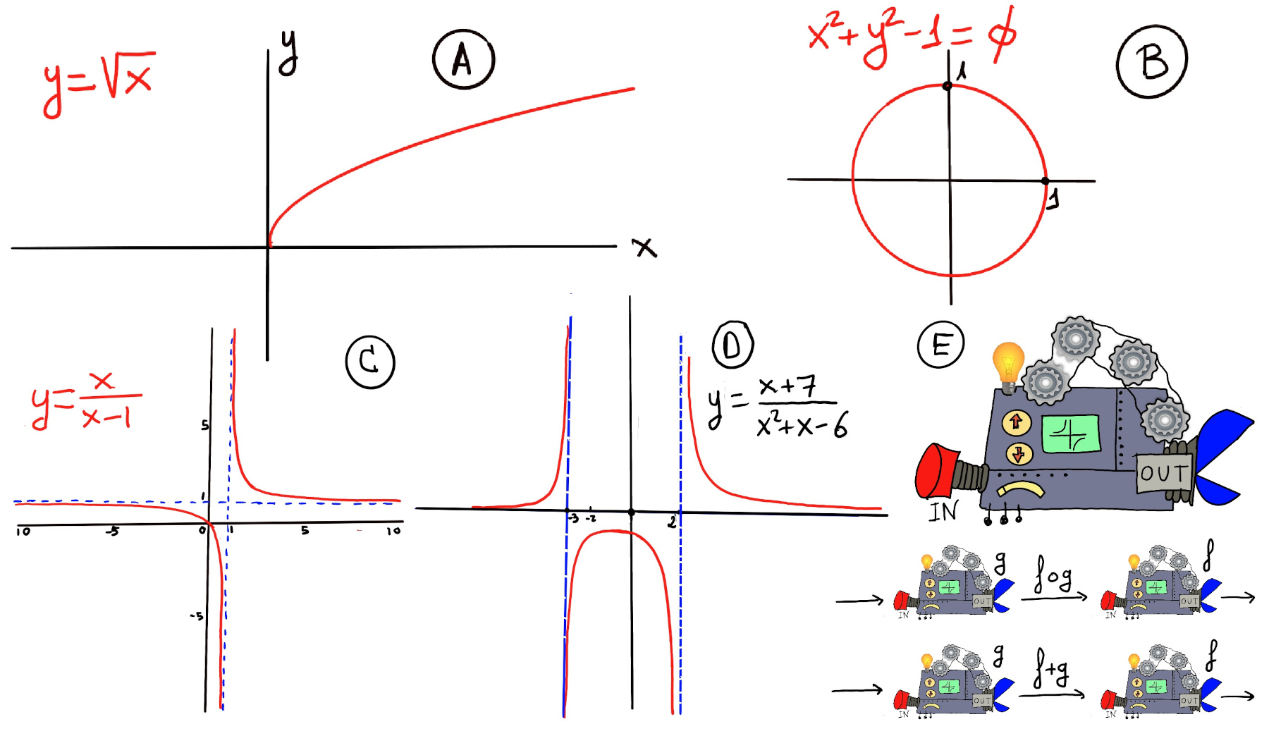
Definition. A function f is a rule, relationship, or correspondence that assigns to each element x in a set D, x ∈ D (called the domain) exactly one element y in a set E, y ∈ E (called the codomain or range).

• The pair (x, y) is denoted as y = f(x) where: x is the independent variable (input) and y is the dependent variable (output). Often, both the domain D and codomain E are the set of real numbers ℝ or subsets of ℝ. A mathematical function can be thought of as a black box (or machine) that takes an input from its domain and produces exactly one output in its codomain. Inside the machine lives a specific rule (formula, procedure, or mapping) that dictates or tells you which output corresponds to each input, and a key property is uniqueness —each input maps to a single, deterministic output. No input can ever produce two different results (Figure E). The function f(x) = x² accepts any real number x (domain: ℝ) and returns exactly one non-negative value x² (output in codomain: [0,∞)). The input 3 always yields 9, never any other value.

• D is the domain, the set of all possible inputs. E is the codomain or range, the set of all possible outputs.

• Key property💡: Each input has exactly one output. (No input is assigned two different outputs — this is the vertical line test!)

• Examples: constant, f(x) = c, horizontal line, slope = 0; linear, f(x) = mx + b, straight line, constant slope m and y-intercept b; quadratic $f(x) = ax^2 + bx + c$, u-shaped or inverted U, opens up (a > 0) or down (a < 0), vertex at x = $\frac{-b}{2a}$, symmetry about vertical axis through vertex; polynomial, $f(x) = a_n x^n + \dots + a_0$, a smooth and continuous curve, n roots (counting multiplicity), end behaviour determined by its leading term $a_n x^n$; exponential function, $f(x) = a \cdot b^x, a \ne 0, b \gt 0$, rapid growth (b > 1) or decay (0 < b < 1); trigonometric functions, $\sin(x), \cos(x), \tan (z)$ oscillatory, periodic behavior (period 2π for sin/cos, π for tan), sin and cos are bounded between -1 and 1, but tan is unbounded; step function $f(x) = \lfloor x \rfloor$, greatest integer ≤ x, constant on intervals [n, n+1), jumps at integers, its graph is a staircase shape; absolute value f(x) = |x|, V-shaped graph, slope changes at 0.

• Functions can be expressed in multiple forms, each useful in different contexts: verbal description, table of values (list of pairs), algebraic formula, graph, piecewise definition, recursive definition, parametric or integral form, and series representation.

• Evaluating a function means finding or computing the output value f(x) for a given input value x. f(x) = $x^2-2x +4, f(2) = 2^2 -2\cdot 2 + 4 = 4 - 4 + 4 = 4, f(0) = 0^2 -2\cdot 0 + 4 = 4, f(1) = 1^2 -2\cdot 1 + 4 = 1 -2 +4 = 3$

• The x-intercept is any point on the graph that intersects or crosses the x-axis. In other words, it is the value of x when the function (y-coordinate or y-value) is zero. The y-intercept is the point where the graph intersects or crosses the y-axis. y-coordinate of the point whose x-coordinate is 0, e.g., 2x - 3y = 6. x-intercept: set y = 0 → 2x = 6 ⇒ x=3, so (3, 0). y-intercept: set x = 0 → −3y = 6 ⇒ y = −2, so (0, −2).

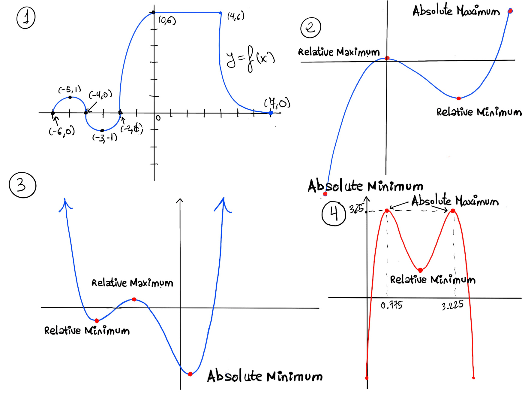
• f is said to have a local or relative maximum at c if there exists an interval (a, b) containing c ($c \in (a, b)$) such that f(c) ≥ f(x) $∀ x \in (a, b) ∩ D$. f is said to have a local or relative minimum at c if there exists an interval (a, b) containing c ($c \in (a, b)$) such that f(c) ≤ f(x) $∀ x \in (a, b) ∩ D$.💡Local extrema can only occur where the function stops rising or falling —either because the derivative is zero, the derivative doesn't exist, or you're at the edge of the domain.

• First Derivative Test. Let f be differentiable on an open interval containing c, except possibly at c itself, and let c be a critical point (so f′(c) = 0 or f′ is undefined). Then:

1. If f′(x) > 0 for x just to the left of c and f′(x) < 0 for x just to the right of c, then f(c) is a local maximum.
2. If f′(x) < 0 for x just to the left of c and f′(x) > 0 for x just to the right of c, then f(c) is a local minimum.
3. If f′(x) does not change sign at c (stays positive or stays negative), then f(c) is not a local extremum.

• Second Derivative Test. If the first derivate of a function at a point c is zero (f'(c) = 0) and the second derivate at this point exists, then: (i) If f''(c) > 0, then f(c) is a local minimum. (ii) If f''(c) < 0, then f(c) is a local maximum. (iii) If f''(c) = 0, the test is inconclusive.
• Vertical asymptotes are vertical lines (perpendicular to the x-axis) of the form x = a (where a is a constant) near which the function grows without bound when x approaches a from at least one side. The line x = a is a vertical asymptote of f if at least one of the one-sided limits is infinite: $\lim_{x \to a^{-}}f(x)=\pm\infty$ or $\lim_{x \to a^{+}}f(x)=\pm\infty$.
• Horizontal asymptotes are horizontal lines (y = c, parallel to the x-axis) that the graph of the function approaches as x grows very large (positively or negatively). In other words, the function values get arbitrarily close to c as long as x is sufficiently large or more formally: $\lim_{x \to \infty}f(x)=c$ and/or $\lim_{x \to -\infty}f(x)=c$.
• A line y = m+b is an oblique (slant) asymptote as $x \to \infty$ if $\lim_{x\to\infty} [f(x) - (mx+b)] = 0.$ This means that the curve of f(x) gets more and more closer to the line y = mx + b as x grows large. For an asymptote y = mx + b as $x \to \infty, m = \lim_{x\to\infty} \frac{f(x)}{x}, b = \lim_{x\to\infty} \bigl(f(x) - m x\bigr)$, provided both limits exist.

Concave Functions

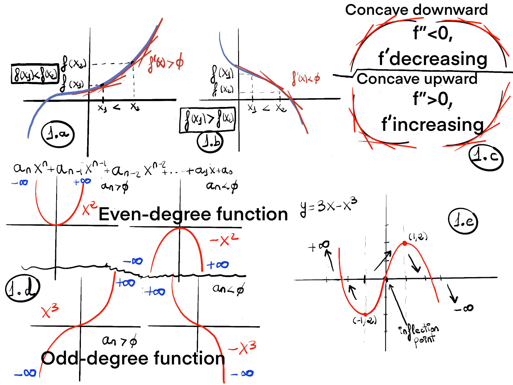
Concavity and inflection points are essential concepts in calculus that describe the curvature of functions. a function’s graph. While monotonicity tells us whether a function is increasing or decreasing, concavity tells us how it increases or decreases —whether the slope itself is increasing or decreasing. Understanding concavity and identifying inflection points provides valuable insights into the behavior of functions.

The concavity of a function describes the direction in which its graph bends (or opens).

• If the graph bends upward, the function is concave up (or convex).
• If the graph bends downward, the function is concave down (often simply called concave).

Geometric Definitions

Definition. A function is concave up or convex on an interval if it curves or bends upwards. Geometrically, this means that the line, segment or chord joining any two points A₁, A₂ on the graph of the function lies above the graph between those points (the midpoint B lies above the corresponding point A₀ of the graph of the function). It means that the function's graph is shaped like a 'U', a bowl, or a smiley face 😃 and lies above its tangent lines on that interval.

Definition. A function is concave down or just concave if it curves or bends downwards. Geometrically, the line, segment or chord joining any two points on the graph lies below the graph between those points. It means that the function's graph is shaped like an upside-down 'U', i.e., '∩', an umbrella, or a frown face 😞 and lies below its tangent lines on that interval.

Formal (Analytic) Definition

Let f be a function defined on an interval [a, b].

• f is concave up or convex on [a, b] if ∀ x₁, x₂ ∈ [a, b] and ∀θ such that 0 < θ < 1, the following inequality holds: f(θx₁ + (1-θ)x₂) ≤ θf(x₁) + (1-θ)f(x₂) where θx₁ + (1-θ)x₂ ∈ (a, b).
• f is concave down on an interval [a, b] if ∀ x₁, x₂ ∈ [a, b], ∀θ such that 0 < θ <1, the following inequality holds: f(θx₁ + (1-θ)x₂) ≥ θf(x₁) + (1-θ)f(x₂) where θx₁ + (1-θ)b ∈ (a, b).

  These inequalities express precisely the idea that the graph lies below (concave up) or above (concave down) its chords.

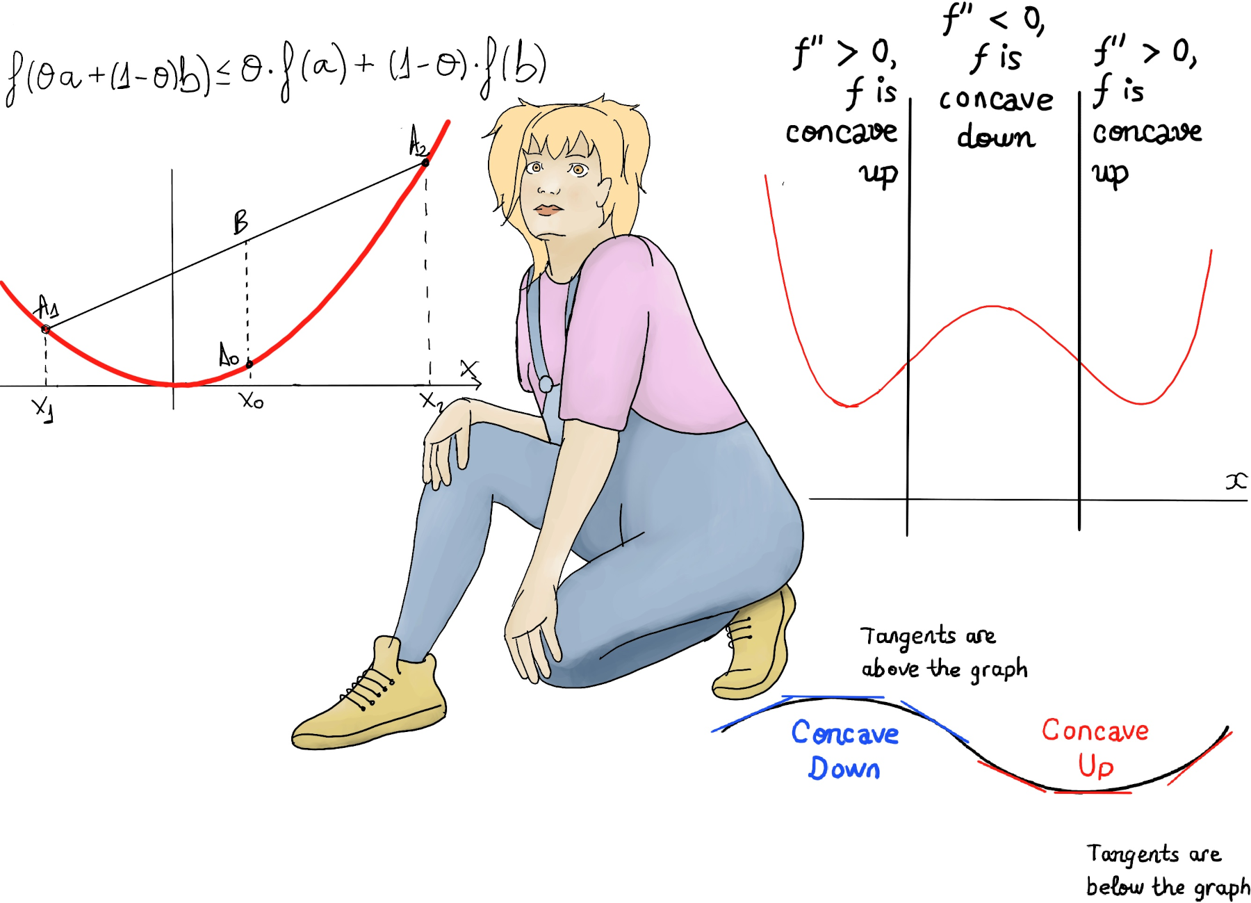
In the graph below (Figure 1):

• The function f is increasing on (-6, -5) ∪ (-3, 0) and decreasing on (-5, -3) ∪ (4, 7).
• It is constant on [0, 4].
• Furthermore, f is concave up on (-4, -2) ∪ (4, 7) and concave down on (-6, -4) ∪ (-2, 0).

Concavity and the Second Derivative

Concavity is directly related to how the derivative of a function behaves.

Concavity relates to the rate of change of a function’s derivative. A function is concave up or convex if its derivative f' is increasing or equivalently, its second derivate f'' is positive. Similarly, f is concave down or concave if its derivative f' is decreasing or equivalently, its second derivate f'' is negative.

f′′(x) > 0 ⇒ f is concave up near x, f′′(x) < 0 ⇒ f is concave down near x.

Example: Quadratic Functions. The equation of a quadratic function is y = ax² + bx + c, where a, b, and c are constants. The graph of a quadratic function is a parabola.

• If a > 0, the parabola opens upward and is concave up.
• If a < 0, the parabola opens downward and is concave down.

Since the second derivative of any quadratic function is just 2a, the sign of “a” completely determines the concavity. If a is positive, f’’ = 2a is positive so the function is concave up, e.g., x² -Figure ii-, 3x² - 4x + 4. If a is negative, f’’ = 2a is negative so the function is concave down, e.g., -x² -Figure ii-, -3x² + 4x + 4.

Inflection Points

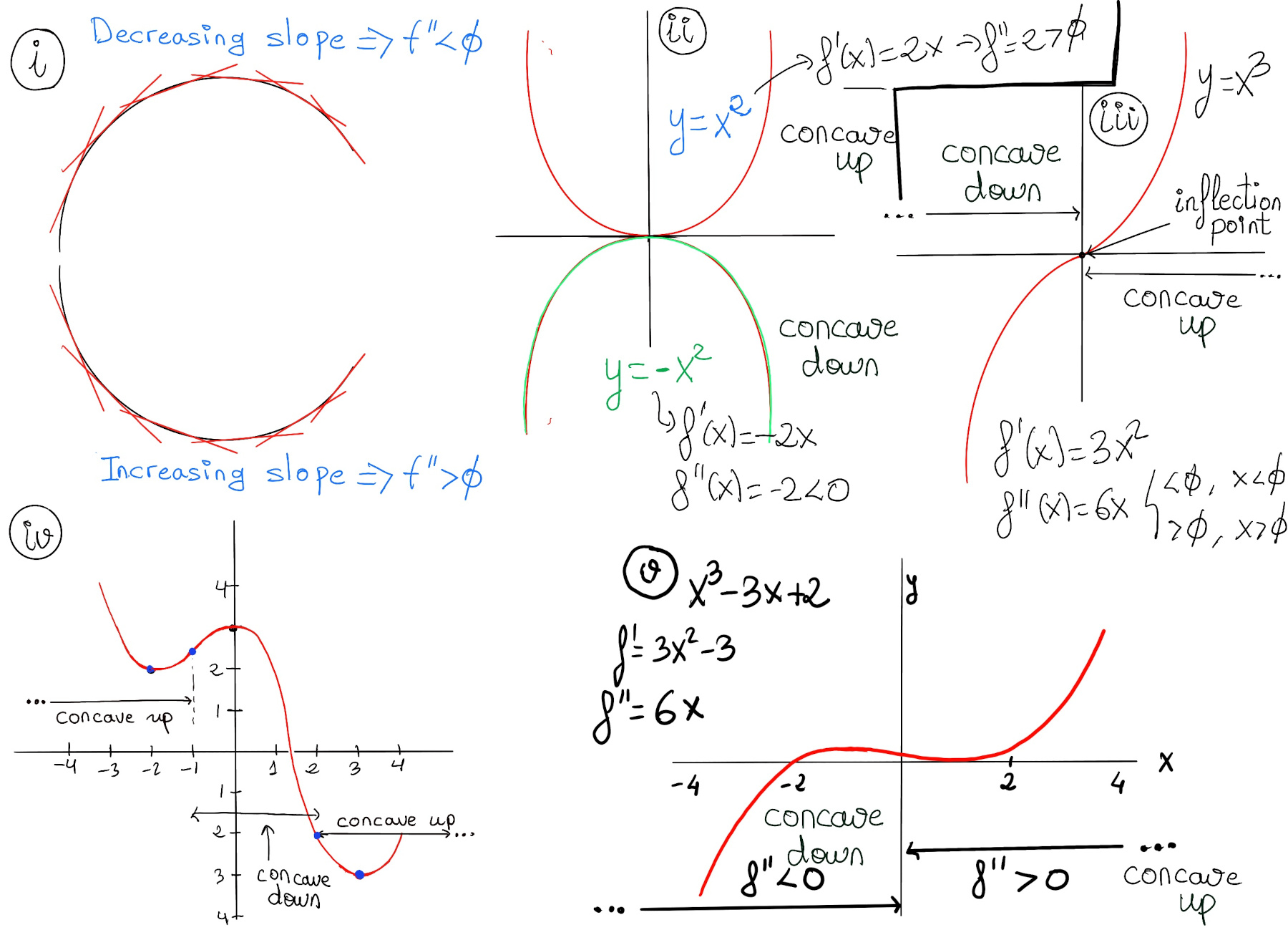
Definition. An inflection point is a point on the graph where the concavity changes, i.e., where the function changes from being concave up to concave down or viceversa.

Analytic Characterization. If f is twice differentiable and has an inflection point at $x_0$, then $f''(x_0) = 0$ or $f''(x_0)$ does not exist. However, this condition alone is not sufficient.

However, it’s important to emphasize that not all points where the second derivative is zero or undefined are inflection points. The concavity must actually change sign across these points for them to be considered inflection points, e.g., $f(x)=x^4, f''(x) = 12x^2$ has f’’(0) = 0. However, $f''(x) = 12x^2 > 0, \forall x \in \mathbb{R}, x \ne 0$, so the concavity is up on both sides of 0 with no sign change. Therefore, x = 0 is not an inflection point.

Equivalently, a differentiable function has an inflection point at $x_0$ if and only if its first derivative f′ has a local extremum at $x_0$: $x_0$ is an inflection point of f ↭ $x_0$ is a local extremum of f'.

Solved examples

• f(x) = x² (Figure ii), f’(x) = 2x, f’’(x) = 2 > 0, f is concave up everywhere. No inflection points (concavity never changes).
• f(x) = -x² (Figure ii), f’(x) = -2x, f’’(x) = -2 < 0, f is concave down everywhere. No inflection points (concavity never changes).
• f(x) = x³ (Figure iii), f’(x) = 3x², f’’(x) = 6x. (i) x > 0 ⇒ f’’(x) > 0, f is concave up; (ii) x < 0 ⇒ f’’(x) < 0, f is concave down. (iii) x = 0 is an inflection point (concavity changes, f is defined at x = 0).
• f(x) = $\frac{1}{x}, f'(x)=\frac{-1}{x^2}, f''(x)=\frac{2}{x^3}$ changes sign at x = 0, but 0 is not an inflection point due to the fact that f is undefined at x = 0. 0 is NOT an inflection point because it must be in the domain!
• f(x) = x³-3x+2 (Figure v), f’(x) = 3x²-3, f’’(x) = 6x. (i) x > 0 ⇒ f’’(x) > 0, f is concave up; (ii) x < 0 ⇒ f’’(x) < 0, f is concave down; (iii) 0 is an inflection point at (0, 2).

• f(x) = 3x -x³ (Figure 1.e). f’(x) = 3 -3x², f’’(x) = -6x.

1. x < 0, f’’(x) > 0 ⇒ f’ is increasing, f is concave up.
2. x > 0, f’’(x) < 0 ⇒ f’ is decreasing, f is concave down.
3. x = 0: Inflection point at (0, 0).

• f(x) = $\frac{x+1}{x+2}$. f’(x) = $\frac{1}{(x+2)^2} \ge 0$, ∀x ∈ ℝ, x ≠ -2 ⇒ f is increasing on both sides of asymptote (-∞, -2) ∪ (-2, ∞). $f''(x) = \frac{-2}{(x+2)^3}$. The plot is shown in Figure 1.a.

1. x < -2 ⇒ f’’(x) > 0, concave up.
2. x > -2 ⇒ f’’(x) < 0, concave down.
3. -2 is not an inflection point because the function is undefined at this value. It is not in the domain.

• f(x)=2x³ −12x² +4x −27, f’(x) = 6x² -24x +4, f’’(x)= 12x -24 = 0 ↭ x = 2.

1. (-∞, 2), e.g., f’’(0) = -24 < 0, f concave down.
2. (2, ∞), e.g., f’’(3) = 36 -24 = 12, f’’(x) > 0, f concave up.
3. x = 2: Inflection point at (2, f(2)) = (2, −43).

• f(x) = sin(x) + cos(x), Domain(f) = [0, 2π]. Compute Derivatives: f’(x) = cos(x) -sin(x), f’’(x) = -sin(x) -cos(x). Find Inflection Points. Set f’’(x) = 0 ↭ -sin(x) = cos(x) ⇒ x = $\frac{π}{4} + \frac{π}{2} = \frac{3π}{4}$ (Quadrant II, where sine is positive and cosine is negative) and $\frac{3π}{4} + π = \frac{7π}{4}$ (Quadrant IV, where sine is negative and cosine is positive). Sign Analysis:

1. (0, $\frac{3π}{4}$), e.g., f’’($\frac{π}{2}$) = -1 < 0, f concave down.
2. ($\frac{3π}{4}, \frac{7π}{4}$), e.g., f’’(π) = 1, f’’(x) > 0, f concave up.
3. ($\frac{7π}{4}, 2π$), e.g., f’’($\frac{11π}{6}$) = -0.366, f’’(x) < 0, f concave down.
4. $x = \frac{3π}{4}$: Inflection point at $(\frac{3π}{4}, 0)$. $x = \frac{7π}{4}$: Inflection point at $(\frac{3π}{4}, 0)$.

• f(x) = $\frac{x^{2}}{1-x^{2}}$. The plot is shown in Figure 1.d.

1. Domain = ℝ - {1, -1}. f(0) = 0.
2. Derivative: f’(x) = $\frac{2x}{(1-x^{2})^{2}}$. Critical points: 0 (f’(x)=0), 1 and -1 (f’ is undefined).
3. Monotonicity: x < -1, f’(x) < 0 ⇒ f decreasing ↘. -1 < x < 0, f’(x) < 0 ⇒ f decreasing ↘. 0 < x < 1, f’(x) > 0 ⇒ f increasing ↗. x > 1, f’(x) > 0 ⇒ f increasing ↗.
4. Second derivative: f’’(x) = $\frac{6x^{2}+2}{(1-x^{2})^{3}}$.
5. Concavity: (i) x < -1, f’’(x) < 0 ⇒ concave down; -1 < x < 1, f’’(x) > 0 ⇒ concave up; x > 1, f’’(x) < 0 ⇒ concave down.
6. 1 and -1 are not inflection points because f is undefined at these points.

• f(x) = ^x⁄_lnx, x > 0. The plot is shown in Figure 1.b.

1. Dom(f) = ℝ⁺ - {0, 1}.
2. Derivative: f’(x) = $\frac{lnx-x(\frac{1}{x})}{(lnx)^{2}}=~ \frac{lnx -1}{(lnx)^{2}}$
3. Critical point: f’(x) = 0 ↭ lnx = 1 ↭ x = e, and f(e) = e.
4. Monotonicity: If 0 < x < 1, f’(x) < 0 ⇒ f is decreasing ↘. 1 < x < e, f’(x) < 0 ⇒ f is decreasing ↘. x > e, f’(x) > 0 ⇒ f is increasing ↗. Hence, f has a local minimum at x = e.
5. Second derivative: f’’(x) = $\frac{\frac{1}{x}(lnx)^{2}-\frac{(lnx-1)2lnx}{x}}{(lnx)^{4}}=~ \frac{\frac{lnx-2(lnx-1)}{x}}{(lnx)^{3}}=~ \frac{2-lnx}{x(lnx)^{3}}$
6. Concavity: If 0 < x < 1, numerator: $2-\ln x=2-(\mathrm{negative})>2>0$, denominator: $x>0, (\ln x)^3<0$, so $x(\ln x)^3<0$ ⇒ f’’(x) < 0 ⇒ concave down. 1 < x < e², $0<\ln x<2$, numerator: $2-\ln x>0$, denominator: $x>0, (\ln x)^3>0 ⇒ x(\ln x)^3>0$ ⇒ f’’(x) > 0 ⇒ concave up. x > e², ln(x) > 2, numerator: 2 -ln(x) < 0, denominator: $x > e^2 >0, (\ln x)^3>0 ⇒ x(\ln x)^3>0$ ⇒ f’(x) < 0 ⇒ concave down.
7. Concavity changes at x = 1 (from down to up), but f is not defined at x = 1, so x = 1 is not an inflection point. Concavity changes at x = $e^2$ (from up to down), and f is defined there. x = $e^2$ is indeed an inflection point.

Bibliography

1. NPTEL-NOC IITM, Introduction to Galois Theory.
2. Algebra, Second Edition, by Michael Artin.
3. LibreTexts, Calculus. Abstract and Geometric Algebra, Abstract Algebra: Theory and Applications (Judson).
4. Field and Galois Theory, by Patrick Morandi. Springer.
5. Michael Penn, and MathMajor.
6. Contemporary Abstract Algebra, Joseph, A. Gallian.
7. YouTube’s Andrew Misseldine: Calculus. College Algebra and Abstract Algebra.
8. MIT OpenCourseWare 18.01 Single Variable Calculus, Fall 2007 and 18.02 Multivariable Calculus, Fall 2007.
9. Calculus Early Transcendentals: Differential & Multi-Variable Calculus for Social Sciences.