Mean Value Theorem for Integrals

Not everything that can be counted counts and not everything that counts can be counted, Albert Einstein.

Quantity has a quality all its own, Joseph Stalin.

Antiderivatives

Antiderivatives are the inverse operation of derivatives and form the foundation of integral calculus.

Given a function $f(x)$, an antiderivative (also known as an indefinite integral), denoted as $F(x)$, is a function that can be differentiated to obtain the original function, i.e., $F'(x) = f(x)$; e.g., $3x^2 - 1$ is the derivative of $x^3 - x + 7$, which means $x^3 - x + 7$ is an antiderivative of $3x^2 - 1$.

Symbolically, the process of finding antiderivatives is called integration, and we write it as: $F(x) = \int f(x)dx$

The Fundamental Theorem of Calculus (Net Change Theorem)

The Fundamental Theorem of Calculus bridges the gap between derivatives and integrals.

It states that the definite integral of a function $f$ over an interval $[a, b]$ is equal to the change in any of its antiderivatives $F$ between the ends of that interval: $\boxed{\int_{a}^{b} f(x)dx = F(b) - F(a) = F(x) \bigg\vert{}_{a}^{b}}$

If we consider $f$ to be a continuous rate of change (meaning $f(x) = F'(x)$), this theorem can be restated as the Net Change Theorem: The definite integral of a rate of change of a function on $[a, b]$ is the total change of the function itself on that interval.

The Second Fundamental Theorem of Calculus. If $f$ is a continuous function and c is a constant, then f has a unique antiderivative A that satisfies $A(c) = 0$, and that antiderivative is given by the rule $A(x) = \int_{c}^{x} f(t)dt$.

The Average Value of a Function

One of the most valuable applications of the definite integral is that it allows us to calculate the average value of a continuous, infinite set of data points over an interval.

When you want to find the average of a discrete set of $n$ numbers (like test scores), you simply add them up and divide by $n$: $\text{AVG} = \frac{y_1 + y_2 + \cdots + y_n}{n}$.

Definition. The average value of a continuous function f(x) over the interval [a, b] is AVG = $\frac{y_1+y_2+···+y_n}{n}$ where $y_1, y_2, \cdots ,y_n$ represent the function values at specific points within the interval [a, b] and n is the total number of points where the function is evaluated within the interval [a, b].

But how do you find the average temperature over a 24-hour period, where the temperature is changing continuously? You can’t just add up an infinite number of points. This is where integrals come in.

Deriving the Formula

Imagine a continuous function $f(x)$ over the interval $[a, b]$. Let’s partition the interval $[a, b]$ into $n$ equally spaced sub-intervals of width $\Delta x$: $\Delta x = \frac{b - a}{n} \implies \frac{1}{n} = \frac{\Delta x}{b - a}$

If we sample one point $x_i$ from each sub-interval, the average of those $n$ sampled values is: $\text{Average of samples} = \frac{f(x_1) + f(x_2) + \cdots + f(x_n)}{n}$

Substituting $\frac{1}{n}$ with $\frac{\Delta x}{b - a}$, we can rewrite this as: $\frac{1}{b - a} \sum_{i=1}^{n} f(x_i)\Delta x$

Notice that $\sum_{i=1}^{n} f(x_i)\Delta x$ is exactly a Riemann sum. As we take more and more samples ($n \to \infty$ and $\Delta x \to 0$), the Riemann sum becomes the definite integral of the function. Therefore, the exact average value is the integral divided by the length of the interval.

The Average Value Theorem

If $f$ is a continuous function on $[a, b]$, then its average (or mean) value on $[a, b]$ is given by: $\boxed{f_{\text{avg}} = \frac{1}{b - a} \int_{a}^{b} f(x)\,dx}$.

Multiplying by $\frac{1}{b-a}$ normalizes the integral (the accumulated area) so the resulting average is completely independent of the interval’s length.

Examples

Here is how the formula works in practice:

• Constant function: Let $f(x) = c$ over $[a, b]$.
  $f_{\text{avg}} = \frac{1}{b-a} \int_{a}^{b} c\,dx = \frac{1}{b-a} \left[ cx \right]_{a}^{b} = \frac{c(b-a)}{b-a} = c$.
  This is completely expected —if the value is always $c$, the average is $c$.

• Quadratic function: Let $f(x) = x^2$ over the interval $[0, 2]$.
  $f_{\text{avg}} = \frac{1}{2-0} \int_{0}^{2} x^2\,dx = \frac{1}{2} \left[ \frac{x^3}{3} \right]_{0}^{2} = \frac{1}{2} \left( \frac{8}{3} \right) = \frac{4}{3}$

• Linear function: Let $f(x) = 2x - 4$ over the interval $[1, 5]$.
  $f_{\text{avg}} = \frac{1}{5-1} \int_{1}^{5} (2x - 4)\,dx = \frac{1}{4} \left[ x^2 - 4x \right]_{1}^{5} = \frac{1}{4} \left( (25 - 20) - (1 - 4) \right) = \frac{1}{4}(5 + 3) = 2$

• Square root function: Let $f(x) = \sqrt{x}$ over the interval $[1, 4]$.
  $f_{\text{avg}} = \frac{1}{4-1} \int_{1}^{4} x^{1/2}\,dx = \frac{1}{3} \left[ \frac{2}{3}x^{3/2} \right]_{1}^{4} = \frac{1}{3} \left( \frac{2}{3}(4^{3/2}) - \frac{2}{3}(1^{3/2}) \right) = \frac{1}{3} \left( \frac{16}{3} - \frac{2}{3} \right) = \frac{14}{9}$

• Trigonometric function: Let $f(x) = \sin(x)$ over the interval $[0, \pi]$.
  $f_{\text{avg}} = \frac{1}{\pi - 0} \int_{0}^{\pi} \sin(x)\,dx = \frac{1}{\pi} \left[ -\cos(x) \right]_{0}^{\pi} = \frac{1}{\pi} ( -\cos(\pi) + \cos(0) ) = \frac{1}{\pi} (1 + 1) = \frac{2}{\pi}$

The Mean Value Theorem for Integrals

The Average Value formula gives us a specific number, $f_{\text{avg}}$. But does the function ever actually hit that exact value?

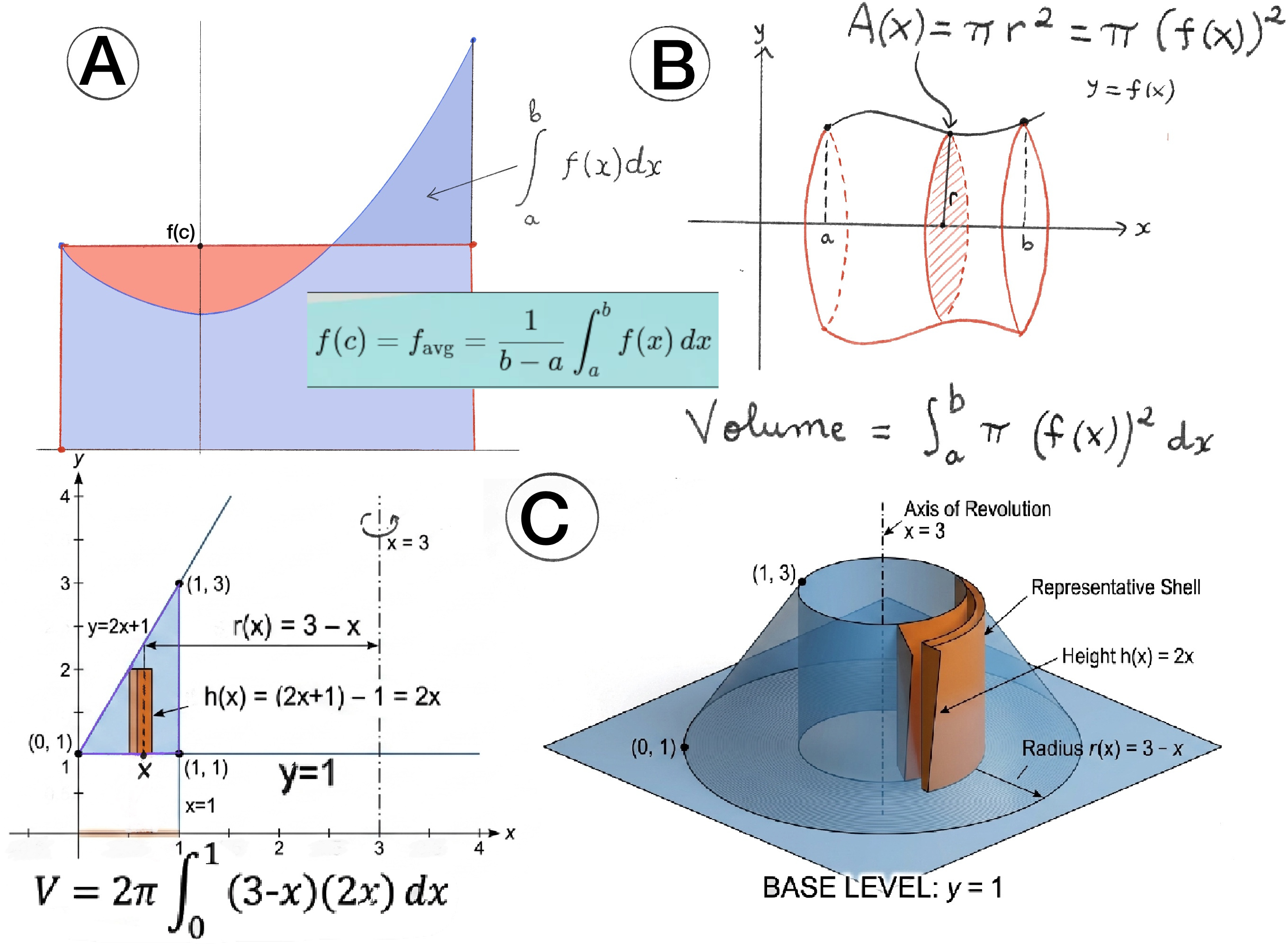
The Mean Value Theorem for Integrals. If $f$ is a continuous function on $[a, b]$, then there exists at least one number $c$ in $[a, b]$ such that: $\boxed{f(c) = f_{\text{avg}} = \frac{1}{b - a} \int_{a}^{b} f(x)\,dx}$ which can be rearranged as: $\int_{a}^{b} f(x)\,dx = f(c)(b - a)$

Geometric Interpretation: The theorem states if f(x) is a continuous function then somewhere in the interval $[a, b]$, the function will take on its average value. Geometrically, this means there is a rectangle with width $(b-a)$ and height $f(c)$ that has the exact same area as the region under the curve $f(x)$, Figure A.

Solved exercises

Average Height of a Semicircle

Problem: Find the average height of a point on the upper half of the unit circle, $y = \sqrt{1 - x^2}$, with respect to the x-axis on the interval $[-1, 1]$.

1. $f_{\text{avg}} = \frac{1}{1 - (-1)} \int_{-1}^{1} \sqrt{1 - x^2}\,dx = \frac{1}{2} \int_{-1}^{1} \sqrt{1 - x^2}\,dx$ (Figure 1.a.).
2. Using trigonometric substitution $x = \sin(\theta), dx = \cos(\theta)d\theta$. Bounds: $x = -1 \implies \theta = \frac{-\pi}{2}; x = 1, \theta = \frac{\pi}{2}$, we get: $\int_{-\frac{\pi}{2}}^{\frac{\pi}{2}} \sqrt{1-\sin^2(\theta)}\cos(\theta)d\theta = \int_{-\frac{\pi}{2}}^{\frac{\pi}{2}} \cos^2(\theta)d\theta$.
   Note: On $\theta \in [-\frac{\pi}{2}, \frac{\pi}{2}]$, we have $\cos(\theta) \gt 0$, so $\sqrt{1-\sin^2(\theta)}= \sqrt{\cos^2(\theta)} = |\cos(\theta)| = \cos(\theta)$. So far, perfect.
3. Using the cosine double-angle identity $\cos(2\theta) = 2\cos^2(θ) -1$, we get: $\frac{1}{2}\int_{-\frac{\pi}{2}}^{\frac{\pi}{2}} (1 + \cos(2\theta))d\theta$.
4. Compute the antiderivative: $\frac{1}{2}(\theta + \frac{1}{2}\sin(2\theta))\bigg|_{-\frac{\pi}{2}}^{\frac{\pi}{2}}$.
5. Evaluate at the bound and multiply by $\frac{1}{2}$: $\frac{1}{2}(\frac{\pi}{2} + \frac{1}{2}\sin(\pi)- (-\frac{\pi}{2} + \frac{1}{2}\sin(-\pi))) = \frac{1}{2}(\frac{\pi}{2}+\frac{\pi}{2})= \frac{\pi}{4}$.

We can solve this geometrically. The integral $\int_{-1}^{1} \sqrt{1 - x^2}\,dx$ represents the area of a semicircle with radius $r=1$. The area of a full circle is $\pi r^2 = \pi$, so the semicircle’s area is $\frac{\pi}{2}$.

Find the average function value for $f(x) = 16 - x^2$ over $[-4, 4]$ and determine the value(s) of $c$ where the function equals its average value

1. First, calculate the average value.
   Because $16 - x^2$ is an even function (symmetric across the y-axis) and the bounds are symmetric $[-4, 4]$, we can integrate from $0$ to $4$ and multiply by 2:
   $f_{\text{avg}} = \frac{1}{4 - (-4)} \int_{-4}^{4} (16 - x^2)\,dx = \frac{1}{8} \cdot 2 \int_{0}^{4} (16 - x^2)\,dx = \frac{1}{4} \int_{0}^{4} (16 - x^2)\,dx$
   $f_{\text{avg}} = \frac{1}{4} \left[ 16x - \frac{x^3}{3} \right]_{0}^{4} = \frac{1}{4} \left( 64 - \frac{64}{3} \right) = \frac{1}{4} \left( \frac{192}{3} - \frac{64}{3} \right) = \frac{1}{4} \left( \frac{128}{3} \right) = \frac{32}{3}$

2. Now, to find $c$, we set $f(x)$ equal to the average value and solve for $x$: $16 - x^2 = \frac{32}{3}$
   $x^2 = 16 - \frac{32}{3} = \frac{48}{3} - \frac{32}{3} = \frac{16}{3}$
   $x = \pm \sqrt{\frac{16}{3}} = \pm \frac{4}{\sqrt{3}} \approx \pm 2.309$

3. Conclusion: Both $c = \frac{4}{\sqrt{3}}$ and $c = -\frac{4}{\sqrt{3}}$ fall within the interval $[-4, 4]$, so there are two points where the function hits its exact average value.

Average Height of a Semicircle (By Arc Length)

Problem: Find the average height of a point on a unit semicircle, evaluated with respect to the arc length $\theta$ (Figure 1.b).

First, let’s establish our variables. On a unit circle (radius $r = 1$), the height of any point $(x, y)$ is simply its y-coordinate, which is given by $y = \sin(\theta)$. Furthermore, the formula for arc length is $\boxed{s = r\theta}$. Since $r = 1$, the arc length $s$ is exactly equal to the angle $\theta$ (measured in radians).

This means integrating with respect to the arc length is exactly the same as integrating with respect to the angle $\theta$ from $0$ to $\pi$, $f_{\text{avg}} = \frac{1}{\pi - 0} \int_{0}^{\pi} \sin(\theta)\,d\theta$

$f_{\text{avg}} = \frac{1}{\pi - 0} \int_{0}^{\pi} \sin(\theta)\,d\theta = \frac{1}{\pi} \left[ -\cos(\theta) \right]_{0}^{\pi} = -\frac{1}{\pi} \left( \cos(\pi) - \cos(0) \right) = -\frac{1}{\pi} (-1 - 1) = -\frac{1}{\pi} (-2) = \frac{2}{\pi}$

Finding the Mean Value of a Parabola

Problem: Find the average function value for $f(x) = (x-5)^2$ over $[4, 7]$ and determine the values for which the function equals its average value.

1. Calculate the Average Value.
   While we can expand $(x-5)^2$ into $x^2 - 10x + 25$ and integrate each term, this often leads to difficult and messy arithmetic with large fractions.

2. Use $u$-substitution. It is much easier, faster, and less prone to errors.
   Let $u = x - 5$, which means $du = dx$.
   Next, change the limits of integration:
   $\star$ Lower bound: $x = 4 \implies u = 4 - 5 = -1$
   $\star$ Upper bound: $x = 7 \implies u = 7 - 5 = 2$
   Now the integral is much simpler: $f_{\text{avg}} = \frac{1}{7 - 4} \int_{-1}^{2} u^2\,du = \frac{1}{3} \left[ \frac{u^3}{3} \right]_{-1}^{2}$
   $f_{\text{avg}} = \frac{1}{3} \left( \frac{2^3}{3} - \frac{(-1)^3}{3} \right) = \frac{1}{3} \left( \frac{8}{3} - \left(-\frac{1}{3}\right) \right) = \frac{1}{3} \left( \frac{9}{3} \right) = \frac{1}{3} (3) = 1$

3. Find $c$ such that $f(c) = f_{\text{avg}}$.
   We know the average value is $1$. The Mean Value Theorem for Integrals guarantees that there is at least one point $c$ in the interval $[4, 7]$ where the function’s output is exactly $1$.
   Let’s find it: $(c - 5)^2 = 1$
   Take the square root of both sides: $c - 5 = \pm\sqrt{1} \implies c - 5 = \pm 1$
   This gives us two possible solutions: $c = 5 + 1 = 6$ and $c = 5 - 1 = 4$

4. Conclusion. Both $c = 4$ and $c = 6$ fall within our closed interval $[4, 7]$ (one is an endpoint, which is perfectly valid, too). Therefore, the function hits its average value at both of these points.

Bibliography

1. NPTEL-NOC IITM, Introduction to Galois Theory.
2. Algebra, Second Edition, by Michael Artin.
3. LibreTexts, Calculus. Abstract and Geometric Algebra, Abstract Algebra: Theory and Applications (Judson).
4. Field and Galois Theory, by Patrick Morandi. Springer.
5. Michael Penn, and MathMajor.
6. Contemporary Abstract Algebra, Joseph, A. Gallian.
7. YouTube’s Andrew Misseldine: Calculus. College Algebra and Abstract Algebra.
8. MIT OpenCourseWare 18.01 Single Variable Calculus, Fall 2007 and 18.02 Multivariable Calculus, Fall 2007.
9. Calculus Early Transcendentals: Differential & Multi-Variable Calculus for Social Sciences.