Mastering the Divergence Theorem: Theory, Intuition, and Worked Examples

All those who seem stupid, they are, and also so are half of those who do not, Quevedo.

The Divergence Theorem (Gauss’s Theorem)

The flux of a vector field $\vec{F}$ across a surface $S$ is defined as the dot product of the vector field and the unit normal vector $\hat{\mathbf{n}}$ to the curve. This is expressed mathematically as $\int_{C} \vec{F} \cdot \hat{\mathbf{n}}ds$.

In vector calculus, calculating the flux of a vector field across a complex 3D surface can be a computationally grueling task involving tedious parameterizations. The Divergence Theorem (also known as Gauss’s Theorem or the Gauss-Green Theorem) provides a brilliant workaround.

It provides a powerful tool for converting the surface integral of a vector field's flux through a closed surface $S$ into a significantly easier triple integral over the solid volume enclosed by that surface (Figure B).

The Statement of the Theorem

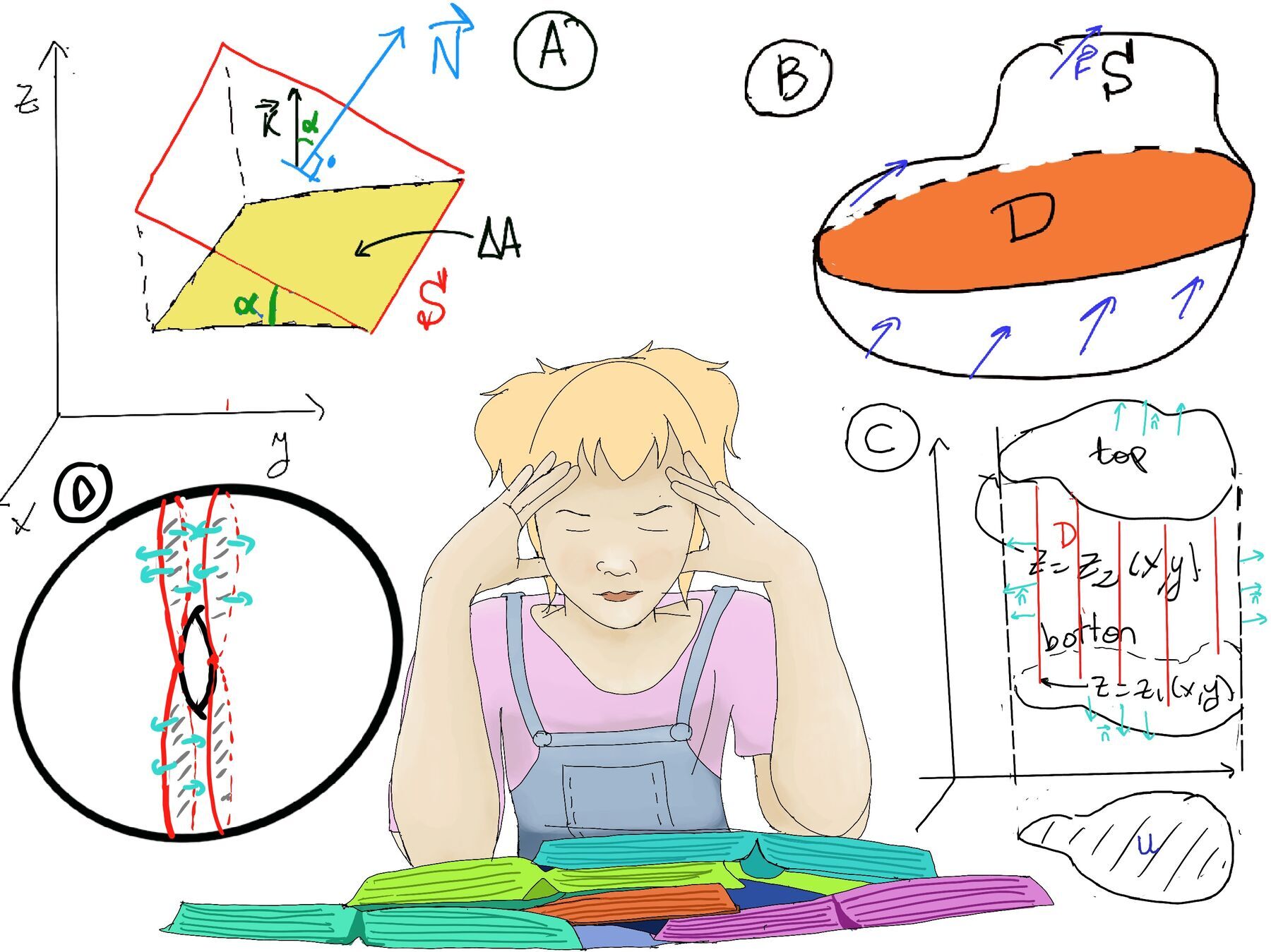
Divergence Theorem. Let $D$ be a bounded, solid region in three-dimensional space, and let $S$ be the closed surface that forms the boundary of $D$. The surface $S$ is oriented with an outward-pointing unit normal vector $\hat{\mathbf{n}}.$ If $\vec{F}$ is a continuously differentiable vector field defined on an open region containing $D$, then the outward flux of the vector field $\vec{F}$ across the closed surface $S$ is given by the triple integral of the divergence of the vector field $\vec{F}$ over the region $D$: $\oiint_S \vec{F} \cdot d\vec{S} = \int \int \int_{D} \operatorname{div}\vec{F} dV \underbrace{=}_\text{Notation} \int \int \int_{D} \nabla \cdot\vec{F} dV$ where:

1. $\vec{F} = \langle P, Q, R \rangle = P\vec{i} + Q\vec{j} + R\vec{k}$ is the vector field, where $P, Q, R$ are the components of the vector field in the $x, y, z$ directions, respectively.
2. The divergence $\nabla \cdot \vec{F}$ is a scalar function that measures the rate at which the vector field $\vec{F}$ is expanding (or contracting) at each point in the region $D$ (the net rate of the outflow of the field).
   It is the dot product of the “del” operator $\nabla = \langle \frac{\partial P}{\partial x}, \frac{\partial Q}{\partial y}, \frac{\partial R}{\partial z} \rangle$ and the vector field.
   $\operatorname{div} \vec{F} = \nabla \cdot \vec{F} = \frac{\partial P}{\partial x} + \frac{\partial Q}{\partial y} + \frac{\partial R}{\partial z} = P_x +Q_y + R_z$ is the divergence of $\vec{F}$
3. $d\vec{S} = \hat{\mathbf{n}}dS$ is the vector surface element where $\hat{\mathbf{n}}$ is the outward-facing unit normal vector.

• Calculate the flux of the vector field $\vec{F} = \langle3xy, y^2, -x^2y^4\rangle$ across the surface of the tetrahedron with vertices $(0, 0, 0), (1, 0, 0), (0, 1, 0)$, and $(0, 0, 1)$ (Refer to Figure ii for a visual representation and aid in understanding it).

The flux of a vector field through a surface is a measure of how much of the field “flows” through the surface. In this problem, instead of directly calculating the flux through each face of the tetrahedron, we can use the Divergence Theorem, which relates the flux through a closed surface to the divergence of the vector field over the volume enclosed by the surface.

$\oiint_S \vec{F} \cdot d\vec{S} = \int \int \int_{D} \operatorname{div}\vec{F} dV \underbrace{=}_\text{Notation} \int \int \int_{D} \nabla \cdot\vec{F} dV$

Step 1. Calculate the Divergence of $\vec{F}$: $\nabla\cdot\vec{F} = P_x +Q_y + R_z$

Given $P = 3xy$, $Q = y^2$, and $R = -x^2y^4$: $\nabla \cdot \vec{F} = \frac{\partial}{\partial x}(3xy) + \frac{\partial}{\partial y}(y^2) + \frac{\partial}{\partial z}(-x^2y^4) = 3y + 2y + 0 = 5y$

Step 2. Set Up the Volume Integral. Next, we need to integrate the divergence $5y$ over the volume $V$ of the tetrahedron. We’ll use Cartesian coordinates for this.

The tetrahedron is bounded by the coordinate planes ($x = 0$, $y = 0$, $z = 0$) and the plane connecting the intercepts, which has the equation $x + y + z = 1$. The limits of integration are:

1. $x$ ranges from $0$ to $1$.
2. For a fixed $x$, $y$ ranges from $0$ to the line $1 - x$.
3. For fixed $x$ and $y$, $z$ ranges from the floor ($z=0$) to the slanted roof ($z = 1 - x - y$).

The volume integral of the divergence over the region D is given by: $\iiint_{D} (\nabla \cdot \vec{F}) \, dV = \int_{0}^{1} \int_{0}^{1-x} \int_{0}^{1-x-y} 5y \, dz \, dy \, dx$

Evaluate the integral

1. The inner integral with respect to $z$: $\int_{0}^{1-x-y} 5ydz = 5yz\bigg|_{0}^{1-x-y} = 5y(1-x-y) = 5y(1-x) - 5y^2$.
2. The middle integral with respect to $y$: $\int_{0}^{1-x} \left( 5y(1-x) - 5y^2 \right) \, dy = \left[ \frac{5(1-x)y^2}{2} - \frac{5y^3}{3} \right]_{0}^{1-x}$
   Substitute $y = 1-x$: $= \frac{5(1-x)(1-x)^2}{2} - \frac{5(1-x)^3}{3} = \frac{5(1-x)^3}{2} - \frac{5(1-x)^3}{3}$
   Finding a common denominator of $6$: $= \frac{15(1-x)^3 - 10(1-x)^3}{6} = \frac{5(1-x)^3}{6}$
3. Finally, the outer integral with respect to $x$. We can use a simple $u$-substitution where $u = 1-x$ and $du = -dx$: $\int_{0}^{1} \frac{5(1-x)^3}{6} \, dx = -\frac{5}{6} \int_{1}^{0} u^3 \, du = \frac{5}{6} \int_{0}^{1} u^3 \, du$
   $= \frac{5}{6} \left[ \frac{u^4}{4} \right]_{0}^{1} = \frac{5}{6} \left( \frac{1}{4} \right) = \frac{5}{24}$

🎉 Conclusion. The total outward flux across the tetrahedron is $\frac{5}{24}$.

• Calculate the flux of the vector field $\vec{F} = \langle x^3+y\sin(z), y^3+z\sin(x), 3z\rangle$ over the surface of the solid bounded by the two hemispheres $z = \sqrt{4-x^2-y^2}, z = \sqrt{1-x^2-y^2}$, and $z = 0$ (Refer to Figure iii for a visual representation and aid in understanding it).

The solid is enclosed by the two hemispheres (a “hollowed out” upper hemisphere. The outer radius is 2, the inner radius is 1) and the disk in the xy-plane, forming a shell-like region.

The flux of a vector field through a surface is a measure of how much of the field “flows” through the surface. Calculating the flux across the inner hemisphere, outer hemisphere, and the flat annular bottom directly would be exhausting. The Divergence Theorem makes this trivial.

$\oiint_S \vec{F} \cdot d\vec{S} = \int \int \int_{D} \operatorname{div}\vec{F} dV \underbrace{=}_\text{Notation} \int \int \int_{D} \nabla \cdot\vec{F} dV$

Step 1. Calculate the Divergence of $\vec{F}$: $\nabla \cdot \vec{F} = \frac{\partial}{\partial x}\left(x^3+y\sin(z)\right) + \frac{\partial}{\partial y}\left(y^3+z\sin(x)\right) + \frac{\partial}{\partial z}(3z)$

$\nabla \cdot \vec{F} = 3x^2 + 3y^2 + 3 = 3(x^2 + y^2 + 1)$

Step 2. Set Up the Volume Integral

The volume integral of the divergence over the region D is given by: $\iiint_{D} (\nabla \cdot \vec{F})dV = \iiint_{D} 3(x^2+y^2+1)dV$

Because our region $D$ is a spherical shell, Cartesian coordinates will be messy. We convert to spherical coordinates $(\rho, \phi, \theta)$: In spherical coordinates, the relationships between Cartesian coordinates and spherical coordinates are:

1. $x = r\cos(\theta) = \rho \sin(\phi)\cos(\theta)$
2. $y = r\sin(\theta) = \rho \sin(\phi)\sin(\theta)$
3. $z = \rho \cos(\phi)$

Therefore, $x^2 + y^2 = \rho^2 \sin^2(\phi)$. The volume differential $dV = \rho^2 \sin(\phi) \, d\rho \, d\phi \, d\theta$. In spherical coordinates, the integrand $3(x^2+y^2+1) = 3(r^2+1) = 3(\rho^2 \sin^2(\phi)+1)$.

The bounds for the solid shell in the upper half-space are:

• $\rho \in [1, 2]$ between the inner and outer spheres.
• $\phi \in [0, \pi/2]$ from the positive $z$-axis down to the $xy$-plane.
• $\theta \in [0, 2\pi]$, a full rotation around the $z$-axis.

The integral becomes: $\iiint_{D} (\nabla \cdot \vec{F})dV = \iiint_{D} 3(x^2+y^2+1)dV = 3\int_{0}^{2\pi} \int_{0}^{\frac{\pi}{2}} \int_{1}^{2} (\rho^2\sin^2(\phi)+1)\rho^2\, \sin(\phi)\, d\rho\, d\phi\, d\theta$.

Because the integrand does not depend on $\theta$, we can immediately integrate $\theta$ to get $2\pi$, leaving: $6\pi \int_{0}^{\pi/2} \int_{1}^{2} \left( \rho^4 \sin^3(\phi) + \rho^2 \sin(\phi) \right) \, d\rho \, d\phi$

Step 3: Evaluate the Integral

First, integrate with respect to $\rho$: $\int_{1}^{2} \left( \rho^4 \sin^3(\phi) + \rho^2 \sin(\phi) \right) \, d\rho = \left[ \frac{\rho^5}{5}\sin^3(\phi) + \frac{\rho^3}{3}\sin(\phi) \right]_{1}^{2}$

$= \left( \frac{32}{5} - \frac{1}{5} \right)\sin^3(\phi) + \left( \frac{8}{3} - \frac{1}{3} \right)\sin(\phi) = \frac{31}{5}\sin^3(\phi) + \frac{7}{3}\sin(\phi)$

Next, integrate with respect to $\phi$: $6\pi \int_{0}^{\pi/2} \left( \frac{31}{5}\sin^3(\phi) + \frac{7}{3}\sin(\phi) \right) \, d\phi$

We can split this into two standard integrals. For the first term, we use the identity $\sin^3(\phi) = \sin(\phi) \sin^2(\phi) = \sin(\phi)(1 - \cos^2(\phi)) = \sin(\phi) - \sin(\phi) \cos^2(\phi)$:

$\int_{0}^{\pi/2} \sin^3(\phi) \, d\phi = \int_{0}^{\pi/2} \sin(\phi) \, d\phi - \int_{0}^{\pi/2} \sin(\phi)\cos^2(\phi) \, d\phi$

$= \Big[ -\cos(\phi) \Big]_{0}^{\pi/2} - \left[ -\frac{\cos^3(\phi)}{3} \right]_{0}^{\pi/2} = (0 - (-1)) - \left( 0 - \left(-\frac{1}{3}\right) \right) = 1 - \frac{1}{3} = \frac{2}{3}$

For the second term: $\int_{0}^{\pi/2} \sin(\phi) \, d\phi = \Big[ -\cos(\phi) \Big]_{0}^{\pi/2} = 1$

Putting it all together: $6\pi \left( \frac{31}{5}\left(\frac{2}{3}\right) + \frac{7}{3}(1) \right) = 6\pi \left( \frac{62}{15} + \frac{35}{15} \right) = 6\pi \left( \frac{97}{15} \right) = \frac{194\pi}{5}$

🎉 Conclusion: The total flux is $\frac{194\pi}{5}$.

• Verify the Divergence Theorem for $\vec{F} = \langle xz, yz, 3z^2 \rangle$ where $D$ is the solid bounded by the paraboloid $z = x^2 + y^2$ and the plane $z = 1$ (Refer to Figure i for a visual representation and aid in understanding it).

The Divergence Theorem (also known as Gauss’s Theorem) is a fundamental result in calculus that relates the flux of a vector field through a closed surface to the divergence of the field within the region bounded by that surface. Let D be the solid enclosed by S. We need to verify that:

$\oiint_S \vec{F} \cdot d\vec{S} = \int \int \int_{D} \operatorname{div}\vec{F} dV \underbrace{=}_\text{Notation} \int \int \int_{D} \nabla \cdot\vec{F} dV$

To “verify” the theorem, we must compute both sides of the equation independently and show they yield the exact same result.

Part 1: The Volume Integral

Step 1: Compute the Divergence

Calculate the Divergence of $\vec{F}$: $\nabla \cdot \vec{F} = \frac{\partial}{\partial x}(xz) + \frac{\partial}{\partial y}(yz) + \frac{\partial}{\partial z}(3z^2) = z + z + 6z = 8z$

Step 2: Volume Integral in Cylindrical Coordinates

The volume integral of the divergence over the region $D$ is given by: $\iiint_{D} (\nabla \cdot\vec{F})dV = \iiint_{D} 8zdV$

To evaluate this, we switch to cylindrical coordinates because the region is symmetric about the $z$-axis. In cylindrical coordinates: $x = r\cos(\theta), y = r\sin(\theta), z = z$, and $dV = r\, dr\, d\theta\, dz$.

The region is bound by the paraboloid $z = r^2$ (where $r = \sqrt{x^2+y^2}$) and the plane $z = 1$. Thus, the limits of integration are: $0 \leq \theta \leq 2\pi$ (the unit circle in the xy-plane; $z = 1$ corresponds to $r^2 = 1$, so $r = 1$, the flat ceiling), and $z = r^2$ from the paraboloid floor ($z = x^2 + y^2 = r^2$).

Now, the volume integral becomes: $\int \int \int_{D} div \vec{F} dV = \int_{0}^{2\pi} \int_{0}^{1} \int_{r^2}^{1} (8z)r\, dz\, dr\, d\theta.$

Step 3: Evaluate

We first integrate with respect to $z$: $\int_{r^2}^{1} 8zrdz = 8r\frac{z^2}{2}\bigg|_{r^2}^{1} = 8r(\frac{1}{2}-\frac{r^4}{2}) = 4r(1-r^4)$.

Next, we integrate with respect to r: $\int_{0}^{1} 4r(1-r^4)dr = 4(\frac{r^2}{2}-\frac{r^6}{6})\bigg|_{0}^{1} = 4(\frac{1}{2}-\frac{1}{6}) = 4(\frac{3}{6}-\frac{1}{6}) = 4\cdot\frac{2}{6} = \frac{8}{6} = \frac{4}{3}$

Finally, integrate with respect to $\theta$: $\int_{0}^{2\pi} \frac{4}{3}d\theta = \frac{4}{3} \cdot 2\pi = \frac{8\pi}{3}$. Thus, the volume integral is $\int \int \int_{D} div \vec{F} dV = \frac{8\pi}{3}$

The volume integral yields $\frac{8\pi}{3}$.

Part 2: The Surface Integral

$\oint_S \vec{F} \cdot d\vec{S} = \oint_S \vec{F} \cdot \hat{\mathbf{n}}dS$

The surface $S$ is composed of two parts:

1. $S_1$: The disk at the top, where $z = 1$.
2. $S_2$: The curved surface of the paraboloid $z = x^2 + y^2$.

Surface Integral over $S_1$ (Top Disk)

On this surface, $z = 1$, so our vector field simplifies to $\vec{F} = \langle x, y, 3 \rangle$.

Because this is a flat horizontal surface acting as the “ceiling” of our volume, the outward unit normal points strictly up: $\hat{\mathbf{n}} = \langle 0, 0, 1 \rangle$.

Therefore, $\iint_{S_1} \vec{F} \cdot \hat{\mathbf{n}} \, dS = \iint_{S_1} \langle x, y, 3 \rangle \cdot \langle 0, 0, 1 \rangle \, dS = \iint_{S_1} 3 \, dS$

This is simply $3$ times the area of the disk. The radius at $z=1$ is $1$, so Area $= \pi(1)^2 = \pi$. $\iint_{S_1} \, dS = 3\pi$

Surface Integral over $S_2$ (Paraboloid)

For the paraboloid $z = x^2 + y^2$, the vector field is: $\vec{F} = \langle xz, yz, 3z^2 \rangle = \langle x(x^2+y^2), y(x^2+y^2), 3(x^2+y^2)^2\rangle $

To find the outward normal vector for a surface defined by $z = g(x,y)$, we write the surface as a level curve $f(x,y,z) = z - x^2 - y^2 = 0$. The gradient vector is $\nabla f = \langle -2x, -2y, 1 \rangle$. However, for the bottom of our solid, the normal must point outward (downward). Thus, we take the negative gradient to get our outward normal vector $\vec{N} = \langle 2x, 2y, -1 \rangle$. (Note: We use $\vec{N} \, dA$ instead of $\hat{\mathbf{n}} \, dS$ to account for the surface parameterization scale factor).

Take the dot product $\vec{F} \cdot \vec{N}$: $\vec{F} \cdot \vec{N} = \langle x(x^2+y^2), y(x^2+y^2), 3(x^2+y^2)^2 \rangle \cdot \langle 2x, 2y, -1 \rangle$

$= 2x^2(x^2+y^2) + 2y^2(x^2+y^2) - 3(x^2+y^2)^2 = (2x^2 + 2y^2)(x^2+y^2) - 3(x^2+y^2)^2 = 2(x^2+y^2)^2 - 3(x^2+y^2)^2 = -(x^2+y^2)^2$

The surface integral over $S_2$ is: $\oint_{S_2} \vec{F} \cdot \hat{\mathbf{N}}dA = \oint_{D} -(x^2+y^2)^2dA$, where $\hat{\mathbf{N}}$ is the outward-pointing normal vector on the surface $S_2$ and $dA$ is the differential area element on the surface.

To simplify the computation, we switch to polar coordinates, where the Cartesian coordinates $(x, y)$ are replaced by polar coordinates $(r, \theta)$, with $r = \sqrt{x^2+y^2}$ and $\theta$ as the angle in the $xy$-plane. In polar coordinates:

• $x^2 + y^2 = r^2$.
• The area element $dA$ in Cartesian coordinates is transformed to $r\, dr\, d\theta$ in polar coordinates.
• The limits of integration for $r$ are from $0$ to $1$ (since the paraboloid surface is bounded by the unit circle in the $xy$-plane), and $\theta$ varies from $0$ to $2\pi$ to cover the entire circle.

Substituting these into the integral, we have: $\oint_{D} -(x^2+y^2)^2dA = \int_{0}^{2\pi}\int_{0}^{1} -(r^2)^2 r\, dr\, d\theta = \int_{0}^{2\pi}\int_{0}^{1} -r^5drd\theta$

Integrate with respect to $r$: $\int_{0}^{1} -r^5dr = -\frac{r^6}{6}\bigg|_{0}^{1} = \frac{-1}{6}$.

Then, integrate with respect to $\theta$: $\oint_{S_2} \vec{F} \cdot \hat{\mathbf{n}}dS = \int_{0}^{2\pi} \frac{-1}{6}d\theta = \frac{-1}{6}\cdot 2\pi = -\frac{\pi}{3}$

Adding the flux from the roof and the bowl: $\oint_S \vec{F} \cdot \hat{\mathbf{n}}dS = \oint_{S_1} \vec{F} \cdot \hat{\mathbf{n}}dS + \oint_{S_2} \vec{F} \cdot \hat{\mathbf{n}}dS = 3\pi -\frac{\pi}{3} = \frac{9\pi}{3}-\frac{\pi}{3} = \frac{8\pi}{3}$.

Conclusion. Since both integral — the volume integral and the surface integral — are equal, the Divergence Theorem is verified for the given vector field and region.

The diffusion equation

The diffusion equation models the process by which quantities such as heat, mass, or charge spread out over time in a medium. It is the mathematical heartbeat of spreading phenomena: from a drop of ink dispersing in a glass of water, to the conduction of heat through a metal engine block, to the way pollutants scatter in the atmosphere.

At its core, diffusion is the spontaneous movement of particles from regions of high concentration to regions of low concentration, driven by the tendency of systems to move toward thermodynamic equilibrium.

Mathematically, if $u(x, y, z, t)$ represents the concentration of a substance (or the temperature) at a spatial point $(x, y, z)$ at a specific time $t$, the isotropic diffusion equation is written as: $\frac{\partial u}{\partial t} = k \nabla^2 u$ where:

• $k$ is the diffusion coefficient (or thermal diffusivity). It dictates how fast the spreading occurs and depends on the nature of the medium (e.g., heat diffuses faster in copper than in wood) and the diffusing substance.
• $u(x,y,z,t)$ is the concentration field.
• $\nabla^2 u$ is the Laplacian of $u$, representing the divergence of the gradient ($\nabla \cdot \nabla u$). It measures how the concentration changes in space.

Before we derive the equation, we must understand the Laplacian, $\nabla^2 u$.

In calculus, the first derivative tells you the slope, and the second derivative tells you the concavity. The Laplacian is the multivariable equivalent of the second derivative: $\nabla^2 u = \frac{\partial^2 u}{\partial x^2} + \frac{\partial^2 u}{\partial y^2} + \frac{\partial^2 u}{\partial z^2}$.

The Laplacian measures how the value of a point compares to the average value of its surrounding neighbors.

• If $\nabla^2 u > 0$, the point is in a “valley” (its concentration is lower than its surroundings), so particles will flow in, causing the concentration to rise over time ($\frac{\partial u}{\partial t} > 0$).
• If $\nabla^2 u < 0$, the point is a “peak” (its concentration is higher than its surroundings), so particles will flow out, causing the concentration to drop ($\frac{\partial u}{\partial t} < 0$).

The Derivation: Flux, Divergence, and Conservation

To rigorously derive the diffusion equation, we combine two fundamental physical principles: Fick’s First Law and the Conservation of Mass.

🧩 Step 1. Fick’s First Law (The Flux).

Let $\vec{F}(x,y,z,t)$ represent the flux of the substance—a vector field describing the direction and magnitude of the flow of particles. Observation dictates that substances naturally flow away from densely packed areas. For instance, if you drop a drop of ink in water, the ink particles will spread out until they are evenly distributed throughout the water.

Mathematically, this is expressed as: $\vec{F} = -k \nabla u$ where $\nabla u$ is the gradient of the concentration, pointing in the direction of the steepest increase. The negative sign flips this vector, ensuring that the flux $\vec{F}$ points toward the steepest decrease in concentration. It indicates that the flux moves from high to low concentration.

🧩 Step 2. The Conservation of Mass (The Continuity Equation).

Imagine an arbitrary, fixed 3D region of space called $D$, bounded by a closed surface $S$. The total amount of substance inside our control volume $D$ is the volume integral of the concentration: $\text{Total Mass} = \iiint_D u \, dV$.

The rate at which this mass changes over time is simply the time derivative of this integral. According to the principle of conservation of mass, if no new material is being created or destroyed inside the volume, the only way the total mass can change is if it flows out through the boundary surface $S$.

We calculate the outward flow using a surface integral of the flux. Therefore, the rate of change of mass equals the negative net outward flux: $\frac{d}{dt} \iiint_D u \, dV = - \iint_S \vec{F} \cdot \hat{\mathbf{n}} \, dS$

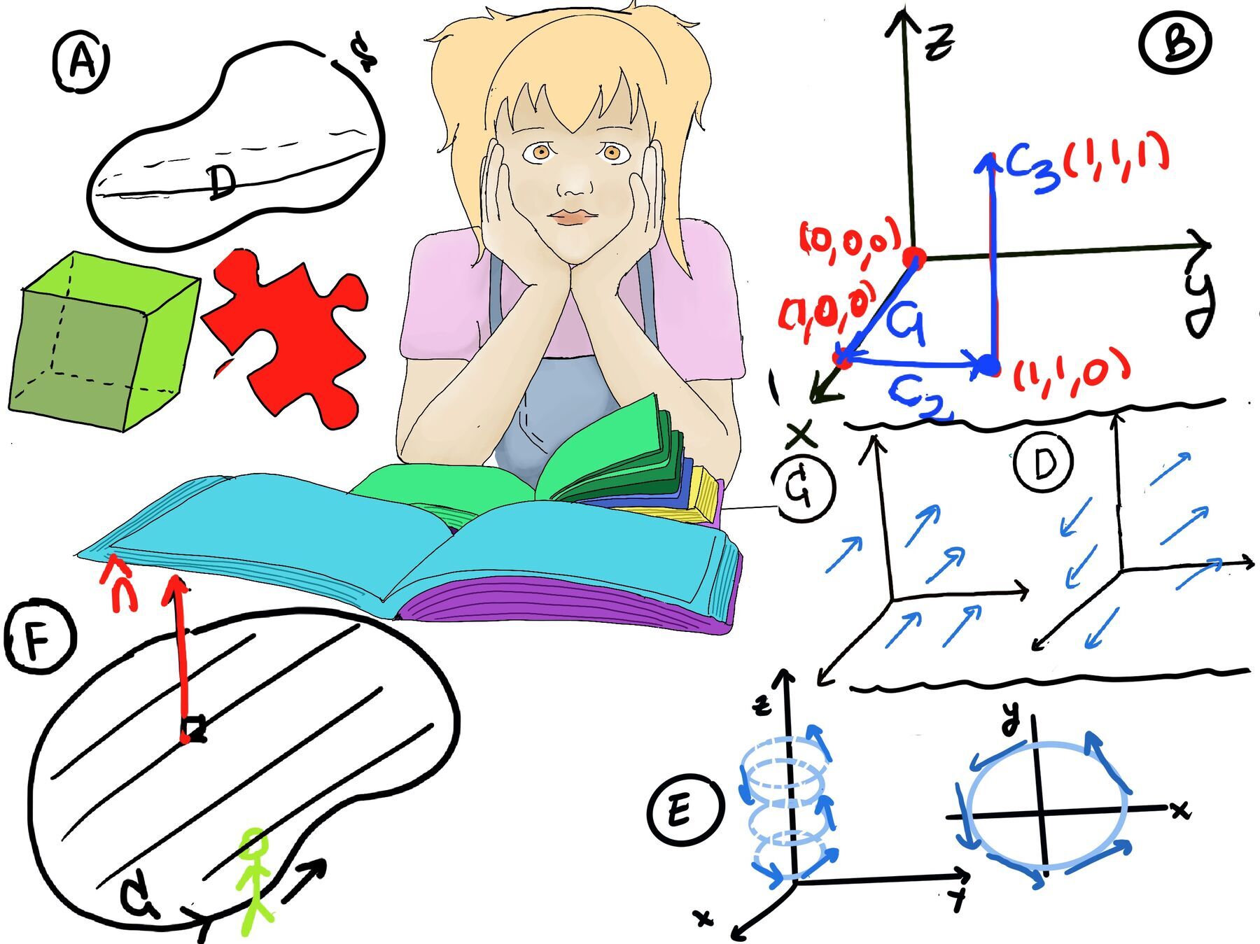
🧩 Step 3. Applying the Divergence Theorem

Dealing with a mix of volume and surface integrals is cumbersome. Fortunately, the Divergence Theorem allows us to translate the surface integral of the flux into a volume integral of the divergence of the flux: $\iint_S \vec{F} \cdot \hat{\mathbf{n}} \, dS = \iiint_D \nabla \cdot \vec{F} \, dV$

Substituting this into our conservation equation yields: $\frac{d}{dt} \iiint_D u \, dV = - \iiint_D \nabla \cdot \vec{F} \, dV$

$\frac{d}{dt} \iiint_D u \, dV$ is the rate of change of total amount of stuff inside the region $D$.

• If $ \nabla \cdot \vec{F} \gt 0$, more mass is leaving the region than entering → total mass decreases.
• If $ \nabla \cdot \vec{F} \lt 0$, more mass is entering the region → total mass increases.
• The minus sign simply encodes that outward flux reduces the amount inside.

🧩 Step 4. Bringing it All Together

Because our control volume $D$ is fixed in space and does not change over time, and the integrand is smooth, we can apply the Leibniz Integral Rule, sliding the time derivative inside the integral as a partial derivative: $\iiint_D \frac{\partial u}{\partial t} \, dV = - \iiint_D \nabla \cdot \vec{F} \, dV$

Obviously, we can move everything to one side of the equation: $\iiint_D \left( \frac{\partial u}{\partial t} + \nabla \cdot \vec{F} \right) dV = 0$

Next, we invoke a powerful mathematical tool known as the Localization Theorem. Because this integral equals zero for any arbitrarily chosen volume $D$, the integrand itself must be identically zero everywhere in the medium. Therefore: $\frac{\partial u}{\partial t} + \nabla \cdot \vec{F} = 0$

If the integrand were nonzero at even one point, you could choose a tiny region around that point and the integral would not be zero.

This is known as the Continuity Equation. Finally, we substitute Fick’s First Law ($\vec{F} = -k \nabla u$, meaning Flux is proportional to the negative gradient; stuff flows from high concentration to low concentration) into the Continuity Equation: $\frac{\partial u}{\partial t} + \nabla \cdot (-k \nabla u) = 0$

Assuming $k$ is a spatial constant, we pull it out of the divergence operator. Recognizing that the divergence of a gradient is the Laplacian ($\nabla \cdot \nabla u = \nabla^2 u$), we arrive at our final result: $\boxed{\frac{\partial u}{\partial t} = k \nabla^2 u}$, which describes how the concentration u changes over time due to diffusion and has a wide range of applications: heat transfer (describe how heat spread through a solid material), chemical diffusion (modelling the spread of pollutants in air or water), biological processes (it helps to understand how substances like oxygen diffuse through tissues) or finance (it models the evolution of prices in markets).

The Laplacian measures how different a point is from its surroundings.

• If the graph of $u$ is shaped like a bowl (concave up, the point is lower than the average of its surroundings) → Laplacian positive → diffusion pushes mass into the point, that is, u increases.
• If the graph of $u$ is shaped like a hill (concave down, the point is higher than the average of its surroundings) → Laplacian negative → diffusion pulls mass mass outward, that is, u decreases.

Boundary Cases and Expansions

The standard diffusion equation is elegant, but the real world is often more complex. Mathematicians and physicists modify this equation to account for various boundary cases:

1. Adding Sources and Sinks
   What if the substance isn’t just diffusing, but is also being actively generated or destroyed? For example, a chemical reaction might consume the substance, or a heated wire might continuously add thermal energy. We account for this by adding a source term $Q(x,y,z,t)$: $\frac{\partial u}{\partial t} = k \nabla^2 u + Q$
   This is known as the inhomogeneous diffusion equation (or Reaction-Diffusion equation), famously used by Alan Turing to explain how animals develop stripes and spots.

2. Anisotropic Diffusion
   Our derivation assumed k was a simple scalar constant, meaning the substance diffuses equally fast in all directions (isotropic). But consider water diffusing through the fibers of a piece of wood: it flows much easier along the grain than across it.
   In this case, the medium is anisotropic. The coefficient k is replaced by a diffusion tensor D (a 3×3 matrix), and the equation becomes: $\frac{\partial u}{\partial t} = \nabla \cdot (\mathbf{D} \nabla u)$

3. The Microscopic Perspective: Brownian Motion
   Why does Fick’s Law work in the first place? At a microscopic level, particles do not “know” they are supposed to move from high to low concentration. Instead, they undergo random walks—Brownian motion. Because there are simply more particles in a region of high concentration, statistically, more particles will randomly wander out of the dense region than into it. The macroscopic diffusion equation is the deterministic limit of trillions of microscopic probabilistic events.

🎲 A simple analogy

Imagine 100 people in Room A and 10 people in Room B. Each minute, every person randomly 🚶 chooses a room to walk into. Even though the choice is random:

• More people will leave Room A (because it has more people).
• Fewer will leave Room B (because it has fewer people).
• After a while, the rooms equalize.

So the diffusion equation is basically the deterministic limit of trillions of random microscopic events.

Broader Applications

The diffusion equation does not just describe heat and smoke; its mathematical structure is a universal tool:

• Finance: The famous Black-Scholes equation, which prices financial options, can be mathematically transformed directly into the heat equation. The “diffusion” of heat maps to the diffusion of financial volatility over time.

• Computer Vision: If you apply a Gaussian Blur filter to an image in Photoshop, the software is practically treating the image’s pixel intensities as a “concentration” and running the 2D diffusion equation forward in time for a few milliseconds. This smooths sharp edges, removes noise, and averages intensities — exactly what diffusion does.

• Probability: The diffusion equation describes the time evolution of the probability density function of a random variable undergoing a random walk (a Wiener process).

Bibliography

1. NPTEL-NOC IITM, Introduction to Galois Theory.
2. Algebra, Second Edition, by Michael Artin.
3. LibreTexts Mathematics, Calculus and Calculus 3e (Apex). Abstract and Geometric Algebra, Abstract Algebra: Theory and Applications (Judson).
4. Field and Galois Theory, by Patrick Morandi. Springer.
5. Michael Penn, and MathMajor.
6. Contemporary Abstract Algebra, Joseph, A. Gallian.
7. YouTube’s Andrew Misseldine: Calculus. College Algebra and Abstract Algebra.
8. MIT OpenCourseWare 18.01 Single Variable Calculus, Fall 2007 and 18.02 Multivariable Calculus, Fall 2007.
9. Calculus Early Transcendentals: Differential & Multi-Variable Calculus for Social Sciences.