Green's theorem

The excitement of learning separates youth from old age. As long as you’re learning, you’re not old, Rosalyn S.Yalow.

Silence is a source of great strength, Lao Tzu.

Vector Fields, Work, and Green’s Theorem

A vector field on a plane is an assignment of a vector $\vec{F}$ to every point $(x, y)$ in a given space. Mathematically, it is expressed as: $\vec{F}(x, y) = \langle M(x, y), N(x, y) \rangle = M\hat{i} + N\hat{j}$ where $M$ and $N$ are scalar functions of $x$ and $y$.

A vector field on a plane can be visualized as a collection of arrows, each attached to a point on the plane. These arrows represent vectors with specific magnitudes and directions. In physics, vector fields often represent forces (like gravity or electromagnetism). If we want to calculate the work done by this force field in moving an object along a specific trajectory $C$, we use a line integral.

The work $W$ done by a force field $\vec{F}$ along a curve $C$ is the integral of the tangential component of the force along the path: $W = \int_C \vec{F} \cdot d\vec{r} = \int_C (M \, dx + N \, dy)$

The Four Faces of Conservative Fields

A vector field is considered conservative if it is the gradient of a scalar potential function $f(x,y)$, meaning $\boxed{\vec{F} = \nabla f}$.

If a vector field is continuous on an open, simply-connected region (a region with no “holes”), the following four properties are mathematically equivalent. If one is true, they are all true:

1. Gradient Field: There exists a scalar potential function $f$ such that $\vec{F} = \nabla f = \langle f_x, f_y \rangle$.
2. Path Independence: The work done by the force in moving an object from point $A$ to point $B$ is identical regardless of the path taken.
3. Conservative Force: The work done by the force around any closed loop $C$ is exactly zero ($\oint_C \vec{F} \cdot d\vec{r} = 0$).
4. Exact Differential: The differential expression $M \, dx + N \, dy$ is exact, meaning it is equal to the total differential $df = f_x \, dx + f_y \, dy$.

For these conservative fields, we can bypass complex line integrals using the Fundamental Theorem of Line Integrals. The work is simply the difference in potential energy between the endpoints: $\boxed{\int_C \nabla f \cdot d\vec{r} = f(B) - f(A)}$

The Component Test for Conservativeness

How do we know if a field is conservative before doing the math? We check the mixed partial derivatives. If $M$ and $N$ have continuous first partial derivatives, the field is conservative if and only if: $\boxed{\frac{\partial M}{\partial y} = \frac{\partial N}{\partial x}}$

But what happens when $\frac{\partial M}{\partial y} \neq \frac{\partial N}{\partial x}$? We can no longer use the Fundamental Theorem of Line Integrals. If the path is a closed loop, we must turn to Green’s Theorem.

Green’s theorem

Green’s Theorem is a profound result in vector calculus. It establishes a direct bridge between a 1D line integral around a simple, closed boundary $C$ and a 2D double integral over the interior region $D$ enclosed by that boundary.

Definition: Positive Orientation

Before stating the theorem, we must define positive orientation. A simple closed curve $C$ is positively oriented if it is traversed counterclockwise. One basic and simple intuition is that if you walk along the curve $C$ in the positive direction $\vec{r(t)}$, the enclosed region $D$ must always remain on your left.

Notation. An integral around a positive oriented, closed curve C can be represented as $ \oint_C Mdx + N dy$.

Green’s Theorem. Let $C$ be a positively oriented (counterclockwise), piecewise smooth, simple closed curve enclosing a region $D$. If $\vec{F} = \langle M, N \rangle$ is a vector field that is defined and has continuous partial derivatives on an open region containing $D$, then Green's Theorem states that: $\oint_C \vec{F} \cdot{} d\vec{r} = \iint_D curl(\vec{F}) dA \iff \oint_C Mdx + N dy = \iint_R (N_x-M_y)dA = \iint_R (\frac{\partial N}{\partial x}-\frac{\partial M}{\partial y})dA$ where:

• $\oint_C \vec{F} \cdot{} d\vec{r}$ represents the work or line integral of the vector field $\vec{F}$ around the curve $C$.
• $\iint_R (\frac{\partial N}{\partial x}-\frac{\partial M}{\partial y})dA$ represents the double integral over the region $R$, with the integrand being the difference between the partial derivatives of N and M respectively.

Indeed we have written $\iint_R \text{curl}(\vec{F}) dA$. Technically, the curl of a vector field is a 3-dimensional vector, not a scalar. We cannot integrate a vector with respect to a scalar area $dA$. In 2D, the quantity $(N_x - M_y)$ is the scalar component of the curl in the $\hat{k}$ direction. It should either be written simply as $(N_x - M_y)$ or formally as $(\nabla \times \vec{F}) \cdot \hat{k}$. I will use the standard $(N_x - M_y)$ to keep it accessible.

The Intuition: Macroscopic vs. Microscopic Circulation

The integrand $\left( \frac{\partial N}{\partial x} - \frac{\partial M}{\partial y} \right)$ represents the 2D scalar curl of the vector field—essentially, the “microscopic circulation” or rotation of the field at a single point.

Imagine filling the region $D$ with infinitely many tiny rotating squares. Where two adjacent squares touch, their internal boundaries flow in opposite directions and perfectly cancel each other out. The only boundaries that don’t cancel out are the ones on the absolute outer edge of the region —the macroscopic curve $C$. Therefore, summing up all the tiny internal rotations (the double integral) is perfectly equivalent to measuring the total circulation along the outer boundary (the line integral).

Green’s Theorem in Action: The Hard Way vs. The Easy Way

To see the sheer power of Green’s Theorem, let’s evaluate a closed-loop line integral using both the traditional parameterization method and Green’s Theorem.

Let $\vec{F} = \langle x^2+y^2, -2xy \rangle$. Evaluate $\oint_C \vec{F} \cdot{} d\vec{r}$ where $C$ and $D$ are the curve and region below respectively (Refer to Figure i for a visual representation and aid in understanding it)

First, let’s check if the vector field $\vec{F}$ is conservative. A vector field is conservative if there exists a scalar potential function $f$ such that $\vec{F} = \nabla f$. A necessary condition for this is that the curl of $\vec{F}$ should be zero, or equivalently: $\frac{\partial M}{\partial y} = \frac{\partial N}{\partial x}$.

However, $\vec{F}$ is not conservative since $\frac{\partial M}{\partial y} = \frac{\partial}{\partial y}(x^2+y^2) = 2y \neq \frac{\partial N}{\partial x} = \frac{\partial}{\partial x}(-2xy) = -2y$. This implies that the line integral $\oint_C \vec{F} \cdot{} d\vec{r}$ depends on the path $C$ and cannot be evaluated using a potential function.

Method 1: The Traditional Way (Direct Evaluation)

The boundary $C$ is composed of two distinct segments, meaning we must compute two separate line integrals:

• Segment $C_1$ (The straight line on the x-axis): From the point $(2, 0)$ to $(-2, 0)$. Parametrization: $-2 \leq t \leq 2, x = -t, y = 0$. Taking differentials: $dx = -dt, dy = 0$.
  $Mdx + Ndy = (x^2 + y^2)dx + (-2xy)dy = (t^2+0)(-dt)+0 = -t^2dt$
• Segment $C_2$ (The lower semicircle): From the point $(-2, 0)$ to $(2, 0)$. Parametrization: $\pi \leq t \leq 2\pi, x = 2\cos(t), y = 2\sin(t)$. Taking differentials: $dx = -2\sin(t)\, dt$ and $dy = 2\cos(t)\, dt$.
  $M\, dx = ((2\cos t)^2 + (2\sin t)^2)(-2\sin t\, dt) = 4(-2\sin t)\, dt = -8\sin t\, dt$
  $N\, dy = -2(2\cos t)(2\sin t)(2\cos t\, dt) = -16\cos^2(t)\sin(t)\, dt$

$\oint_C \vec{F} \cdot{} d\vec{r} = \oint_{C_1} \vec{F} \cdot{} d\vec{r} + \oint_{C_2} \vec{F} \cdot{} d\vec{r}$

$-\int_{-2}^{2} t^2dt + \int_{\pi}^{2\pi} (-8\sin(t)-16\cos^2(t)\sin(t))dt$

$\int_{-2}^{2} t^2dt = \frac{t^3}{3}\bigg|_{-2}^{2} = \frac{8}{3}-(\frac{-8}{3}) = \frac{16}{3}$

$\int_{\pi}^{2\pi} (-8\sin(t)-16\cos^2(t)\sin(t))dt = \int_{\pi}^{2\pi} -8\sin(t)dt -\int_{\pi}^{2\pi} 16\cos^2(t)\sin(t)dt$

$\int_{\pi}^{2\pi} -8\sin(t)dt = -8·[-cos(t)]\bigg|_{\pi}^{2\pi} = 8[cos(2\pi)-cos(\pi)] = 8·[1-(-1)] = 16.$

$\int_{\pi}^{2\pi} -16cos^2(t)sin(t)dt$. Using substitution: $u = \cos(t), du = -\sin(t)dt$. Limits of integration:$t = \pi \implies u = \cos(\pi) = -1, t = 2\pi \implies u = \cos(2\pi) = 1$

Thus, $= 16\int_{-1}^{1} u^2du = \frac{u^3}{3}\bigg|_{-1}^{1} = \frac{16}{3}[1^3-(-1)^3] = \frac{16}{3}·2 = \frac{32}{3}$

$\int_{\pi}^{2\pi} (-8\sin(t)-16cos^2(t)sin(t))dt = \int_{\pi}^{2\pi} -8\sin(t)dt -\int_{\pi}^{2\pi} 16cos^2(t)sin(t)dt = 16 + \frac{32}{3} = \frac{48}{3} + \frac{32}{3} = \frac{80}{3}$

$\oint_C \vec{F} \cdot{} d\vec{r} = -\int_{-2}^{2} t^2dt + \int_{\pi}^{2\pi} (-8\sin(t)-16cos^2(t)sin(t))dt = \frac{-16}{3}+ \frac{80}{3} = \frac{64}{3}$

Method 2: Applying Green’s Theorem

That was grueling. Let’s try Green’s Theorem instead. The region $D$ is the lower half-disk of radius 2.

Green’s Theorem states that for a vector field $\vec{F} = \langle M, N \rangle$, the line integral around a simple, closed curve $C$ can be related to a double integral over the region $R$ enclosed by $C$: $\oint_C \vec{F} \cdot{} d\vec{r} = \iint_R (\frac{\partial N}{\partial x}-\frac{\partial M}{\partial y})dA$

$\iint_R (\frac{\partial N}{\partial x}-\frac{\partial M}{\partial y})dA = \iint_R (-2y-2y)dA = -4\iint_R ydA$

Because $D$ is a semicircle, we immediately switch to polar coordinates ($y = r\sin\theta$, $dA = r\, dr\, d\theta$):
$\star$ $r$ ranges from $0$ to $2$.
$\star$ $\theta$ ranges from $\pi$ to $2\pi$ (the bottom half of the plane).

$\iint_D -4(r\sin\theta)(r\, dr\, d\theta) = -4 \int_{\pi}^{2\pi} \int_0^2 r^2 \sin\theta \, dr\, d\theta$

Because the boundaries are constants, we can separate the integrals: $-4 \left( \int_0^2 r^2 \, dr \right) \left( \int_{\pi}^{2\pi} \sin\theta \, d\theta \right)$

Evaluate the $r$ integral: $\int_0^2 r^2 \, dr = \left[ \frac{r^3}{3} \right]_0^2 = \frac{8}{3}$

Evaluate the $\theta$ integral: $\int_{\pi}^{2\pi} \sin\theta \, d\theta = \left[ -\cos\theta \right]_{\pi}^{2\pi} = -\cos(2\pi) - (-\cos(\pi)) = -1 - (1) = -2$

Multiply it all together: $\oint_C \vec{F} \cdot d\vec{r} = -4 \left(\frac{8}{3}\right) (-2) = \frac{64}{3}$

In just four lines of basic calculus, Green’s Theorem generated the exact same result ($\frac{64}{3}$) that took a page of complex trigonometric substitutions to solve traditionally.

Applying Green’s Theorem to Solve a Line Integral

• Evaluate $\oint_C xy\,dx + x^2y^3\,dy$ where $C$ is a triangle with vertices $(0, 0)$, $(1, 0)$, and $(1, 2)$ with positive orientation (Figure 1).

1. Identify the Vector Field and Partial Derivatives.
   $\oint_C xydx + x^2y^3dy = $[Using Green’s Theorem (the curve does satisfy the required conditions), we can convert the line integral around the closed curve $C$ to a double integral over the region $R$ enclosed by $C$. Green’s Theorem states: $\oint_C Mdx + Ndy = \iint_R (N_x-M_y) dA$] = $\iint_R (N_x-M_y) dA$. The vector field is $\vec{F} = \langle xy, x^2y^3 \rangle$, meaning $M = xy$ and $N = x^2y^3$. We first compute the necessary partial derivatives:
   $\frac{\partial N}{\partial x} = \frac{\partial}{\partial x}(x^2y^3) = 2xy^3$
   $\frac{\partial M}{\partial y} = \frac{\partial}{\partial y}(xy) = x$
   Thus, the integrand for our double integral is $(N_x - M_y) = 2xy^3 - x$.

2. Define the Region $R$ The region $R$ is a right triangle.
   To set up our double integral, we need to define the boundaries.
   The $x$-values range from $0$ to $1$.
   For any given $x$, the $y$-values range from the $x$-axis ($y=0$) up to the hypotenuse.
   The line connecting $(0,0)$ and $(1,2)$ has a slope of $m = 2/1 = 2$, so its equation is $y = 2x$.
   Our inequalities are $0 \le x \le 1$ and $0 \le y \le 2x$.

3. Evaluate the Double Integral. Applying Green’s Theorem: $\oint_C xy\,dx + x^2y^3\,dy = \int_0^1 \int_0^{2x} (2xy^3 - x) \,dy\,dx$.
   We evaluate the inner integral with respect to $y$: $\int_0^{2x} (2xy^3 - x) \,dy = \left[ 2x\left(\frac{y^4}{4}\right) - xy \right]_{y=0}^{y=2x}$
   $= \left( \frac{x(2x)^4}{2} - x(2x) \right) - (0) = \frac{16x^5}{2} - 2x^2 = 8x^5 - 2x^2$
   Now, evaluate the outer integral with respect to $x$: $\int_0^1 (8x^5 - 2x^2) \,dx = \left[ \frac{8x^6}{6} - \frac{2x^3}{3} \right]_0^1 = \left[ \frac{4x^6}{3} - \frac{2x^3}{3} \right]_0^1 = \frac{4}{3} - \frac{2}{3} = \frac{2}{3}$

• Evaluate $\oint_C ye^{-x}\,dx + \left(\frac{1}{2}x^2 - e^{-x}\right)\,dy$ where $C$ is a circle of radius 1 centered at $(2, 0)$, oriented counterclockwise.

1. The integral involves the vector field $\vec{F}= \langle M, N \rangle$ where $M=ye^{-x}, N=(\frac{1}{2}x^2-e^{-x})$

2. Apply Green’s Theorem. Green’s Theorem relates the line integral around the closed curve C to a double integral over the region R enclosed by C: $\oint_C Mdx + Ndy = \iint_R (\frac{\partial N}{\partial x}-\frac{\partial M}{\partial y})dA$

3. Calculate the partial derivatives: $N_x = \frac{\partial}{\partial x}(\frac{1}{2}x^2-e^{-x}) = x+e^{-x}, M_y = \frac{\partial}{\partial y}(ye^{-x})=e^{-x}$

4. Set Up the Double Integral. Using Green’s Theorem: $\oint_C ye^{-x}dx + (\frac{1}{2}x^2-e^{-x})dy = \iint_R (x+e^{-x}-e^{-x}) dA =[\text{This simplifies to:}] \iint_R x dA$

We could set up a shifted polar coordinate integral, but there is a much faster way.

Recall the formula for the $x$-coordinate of the center of mass (the centroid, denoted $\bar{x}$) for a region of uniform density: $\bar{x} = \frac{1}{\text{Area}(R)} \iint_R x \,dA$

By multiplying both sides by the Area, we reveal a brilliant shortcut: $\iint_R x \,dA = \bar{x} \cdot \text{Area}(R)$

Since the region $R$ is a perfect circle centered at $(2,0)$, its geometric center $\bar{x}$ is simply $2$. Its area is $\pi r^2 = \pi(1)^2 = \pi$. Therefore: $\iint_R x \,dA = (2) \cdot (\pi) = 2\pi$. No actual integration is required!

• Evaluate $\oint_C y^3dx - x^3dy$ where $C$ is the positively oriented (counterclockwise) circle of radius 2 centered at the origin.

1. Identify the Vector Field.
   The vector field $\vec{F}$ associated with this line integral can be expressed as: $\vec{F} = \langle M, N \rangle = \langle y^3, - x^3 \rangle$.
   Apply Green’s Theorem. Green’s Theorem relates the line integral around the closed curve $C$ to a double integral over the region $R$ enclosed by $C$: $\oint_C Mdx + Ndy = \iint_R (\frac{\partial N}{\partial x}-\frac{\partial M}{\partial y})dA$. Here, the curve C is a circle, which is a simple closed curve, so Green’s Theorem applies.
   $\oint_C y^3dx - x^3dy = \oint_C Mdx + Ndy = \iint_R (N_x-M_y) dA$ where $M=y^3, N=-x^3$.

2. Compute the Partial derivatives. $N_x = \frac{\partial}{\partial x}(-x^3) = -3x^2, M_y = \frac{\partial}{\partial y}(y^3)=3y^2$
   Thus, the integrand for the double integral is: $N_x-M_y = -3x^2-3y^2$

3. Set up the Double Integral. $\oint_C y^3dx - x^3dy = \iint_R curl(\vec{F}) dA = \iint_R (N_x-M_y) dA = \iint_R (-3x^2-3y^2)dA$ where the region $R$ is the disk of radius 2 centered at the origin.

4. Convert to Polar Coordinates.
   Our integral is $\iint_R -3(x^2 + y^2) \,dA$ over a disk of radius 2.
   Integrating this in Cartesian coordinates ($y$ from $-\sqrt{4-x^2}$ to $\sqrt{4-x^2}$) would be an absolute nightmare. Because the region is a centered circle, we switch to polar coordinates: $x = r\cos(\theta), y = r\sin(\theta)$.
   $x^2 + y^2 = r^2, dA = r \,dr \,d\theta$
   Limits: $0 \le r \le 2$ and $0 \le \theta \le 2\pi$.
   The integral becomes: $\iint_R -3(r^2) \,r \,dr \,d\theta = -3 \int_0^{2\pi} \int_0^2 r^3 \,dr \,d\theta$

5. Evaluate.
   We evaluate the inner integral first: $\int_{0}^{2} r^3dr = \frac{r^4}{4}\bigg|_{0}^{2} = \frac{2^4}{4} = 4$
   Now, evaluate the outer integral: $-3 \int_{0}^{2\pi} \int_{0}^{2} r^3drd\theta = -3\int_{0}^{2\pi} 4d\theta = -3·4θ\bigg|_{0}^{2\pi} = -3·(8\pi -0) = -24\pi$
   Final Answer: $\oint_C y^3dx - x^3dy = -24\pi$

• Evaluate $\oint_C x^2y\,dx + (y-3)\,dy$ where $C$ is a rectangle with vertices $(1, 1)$, $(4, 1)$, $(4, 5)$, and $(1, 5)$ oriented counterclockwise. (Figure 2).

1. Identify the Region and the Vector Field. Here, $C$ is a closed curve representing the boundary of the rectangle, and it is oriented counterclockwise. The vector field $\vec{F} = \langle M, N \rangle = \langle x^2y, y-3\rangle$.
   The boundaries of this rectangular region can be described by the inequalities: $1 \leq x \leq 4$ and $1 \leq y \leq 5$.
2. Apply Green’s Theorem. Green’s Theorem (the curve does satisfy the required conditions) relates the line integral around the closed curve $C$ to a double integral over the region $R$ enclosed by $C$: $\oint_C Mdx + Ndy = \iint_R (\frac{\partial N}{\partial x}-\frac{\partial M}{\partial y})dA$ where $M=x^2y, N=y-3$. The region $R$ is the interior of the rectangle $C$ encloses.
3. Compute the partial derivatives: $N_x = \frac{\partial}{\partial x}(y-3) = 0, M_y = \frac{\partial}{\partial y}(x^2y)=x^2$
4. Set up the Double Integral.
   Thus, the integrand for the double integral is: $N_x-M_y = 0 - x^2 = -x^2.$
   The double integral over the region R becomes: $\iint_R (N_x-M_y) dA = \iint_R -x^2dA = \int_{1}^{5}(\int_{1}^{4} -x^2dx)dy.$
5. Evaluate the Double Integral.
   Evaluate the inner integral first: $\int_{1}^{4} -x^2dx = \frac{-x^3}{3}\bigg|_{1}^{4} = -(\frac{4^3}{3}-\frac{1^3}{3}) = -(\frac{64}{3}-\frac{1}{3}) = \frac{-63}{3} = -21$
   Now, evaluate the outer integral: $\iint_R (N_x-M_y) dA = \iint_R -x^2dA = \int_{1}^{5}(\int_{1}^{4} -x^2dx)dy = \int_{1}^{5} -21dy = -21y\bigg|_{1}^{5} = -21(5-1) = -21·4 = -84.$
   $\oint_C x^2ydx + (y-3)dy= -84.$

What happens if we apply Green’s Theorem to a conservative vector field?

By definition, if a vector field $\vec{F}$ is conservative, its mixed partial derivatives are equal ($N_x = M_y$).

If we plug this into Green’s Theorem for any closed loop $C$: $\oint_C M\,dx + N\,dy = \iint_R (N_x - M_y) \,dA = \iint_R (0) \,dA = 0$. This elegantly proves one of the fundamental rules of vector calculus: the work done by a conservative vector field around any closed loop is always zero. If $N_x = M_y$, don’t bother setting up bounds or polar coordinates —the answer is immediately zero!

Handling Clockwise Orientation

By definition, Green’s Theorem requires the boundary curve $C$ to be traversed counterclockwise. If a problem provides a curve with clockwise (negative) orientation, we can still use Green's Theorem, but we must multiply the resulting double integral by $-1$.

• Evaluate $\oint_C (x^5 + 3y)dx + (2x - e^{y^3})dy$ where $C$ is the circle $(x-1)^2 + (y-5)^2 = 4$ oriented clockwise.

1. Apply Green’s Theorem. Green’s Theorem relates the line integral around the closed curve $C$ to a double integral over the region $R$ enclosed by $C$: $\oint_{C} Mdx + Ndy = \iint_R (\frac{\partial N}{\partial x}-\frac{\partial M}{\partial y})dA$
2. Identify our components and compute the partial derivatives.
   $M = x^5 + 3y \implies \frac{\partial M}{\partial y} = 3$.
   $N = 2x - e^{y^3} \implies \frac{\partial N}{\partial x} = 2$
3. Set up the Double Integral.
   The integrand for our double integral is $(N_x - M_y) = 2 - 3 = -1$.
   Because the curve is oriented clockwise, we introduce a negative sign to Green’s Theorem: $-\iint_R (\frac{\partial N}{\partial x}-\frac{\partial M}{\partial y})dA$
   Substituting our integrand: $-\iint_R(2 -3)dA = \iint_R dA$.
4. Notice that the integral simplified to $\iint_R dA$, which is exactly the formula for the geometric area of the region $R$. Since the region is a circle of radius 2 (derived from the equation $(x-1)^2 + (y-5)^2 = 2^2$), its area is simply $\pi r^2$.
   Therefore, $\iint_R dA = \pi(2)^2 = 4\pi$

Regions with Holes (Multiply Connected Domains)

Green’s Theorem works on regions with holes, like an annulus (a ring shape), provided we are careful with the orientation of the boundaries.

• Evaluate $\oint_C (x^3 - y^3)dx + (x^3+y^3)dy$ if $C$ is the boundary of the region between the circles $x^2+y^2 = 1$ and $x^2+y^2 = 9$.

1. Understanding the region.
   The region $R$ is the annular region (a ring-shaped region) between the two circles $x^2+y^2 = 1$ (a smaller circle with radius 1) and $x^2+y^2 = 9$ (a larger circle with radius 3). The curve $C$ is the boundary of this region, consisting of two circular paths: one for the outer boundary (radius 3) and one for the inner boundary (radius 1) (Refer to Figure ii for a visual representation and aid in understanding it).
   The rule for positive orientation in Green’s Theorem is that the region $R$ must always be on your left as you traverse the boundary.
   To keep the ring on your left while walking along the outer circle, you must walk counterclockwise. To keep the ring on your left while walking along the inner circle, you must walk clockwise.
   Effectively, when applying Green’s Theorem, the integral over the region R should consider the area of the region enclosed by the outer circle minus the area of the region enclosed by the inner circle.
   Why does this work? Imagine making a thin “slice” through the ring from the outer edge to the inner edge. If you traverse the outer boundary, walk down the slice, traverse the inner boundary clockwise, and walk back out the slice, the two paths along the slice cancel each other out. This turns the ring into a single, simply connected region where Green’s Theorem flawlessly applies!

2. Apply Green’s Theorem.
   Green’s Theorem relates the line integral around a positively oriented (counterclockwise) curve $C$ to a double integral over the region $R$ enclosed by $C$: $\oint_{C} Mdx + Ndy = \iint_R (\frac{\partial N}{\partial x}-\frac{\partial M}{\partial y})dA$.

3. Identify and compute our partial derivatives:
   $M = x^3 - y^3 \implies M_y = -3y^2$
   $N = x^3 + y^3 \implies N_x = 3x^2$.

4. Set Up the Double Integral: $N_x - M_y = 3x^2 - (-3y^2) = 3(x^2 + y^2)$
   $\iint_R (\frac{\partial N}{\partial x}-\frac{\partial M}{\partial y})dA = \iint_R (3x^2+3y^2)dA$.
   Because $R$ is an annular region, we shift to polar coordinates where $x = r\cos(\theta), y = r\sin(\theta), x^2 + y^2 = r^2$ and $dA = r \, dr \, d\theta$.
   Therefore, the integral becomes, $\iint_R 3(x^2+y^2)dA = \int_{0}^{2\pi} \int_{1}^{3} 3r^2 rdrd\theta = 3\int_{0}^{2\pi} \int_{1}^{3} r^3drd\theta$

5. Evaluate the integral:
   Inner (or radial) integral: $\int_{1}^{3} r^3dr = \frac{r^4}{4}\bigg|_{1}^{3} = \frac{3^4}{4}-\frac{1}{4} = \frac{81}{4}-\frac{1}{4} = \frac{80}{4} = 20$
   Outer (or angular) integral with respect to $\theta$: $\iint_R 3(x^2+y^2)dA = 3\int_{0}^{2\pi} 20d\theta = 3\cdot 20 \theta \bigg|_{0}^{2\pi} = 3\cdot 20 \cdot 2\pi = 120\pi$.
   Thus, the value of the line integral is $\oint_C (x^3 - y^3)dx + (x^3+y^3)dy = 120\pi$

Green’s theorem proof

Green’s Theorem is a fundamental result in vector calculus that establishes a relationship between a line integral around a simple closed curve $C$ and a double integral over the region $R$ enclosed by $C$. Specifically, Green’s Theorem states that: $\oint_C Mdx + Ndy = \iint_R (\frac{\partial N}{\partial x}-\frac{\partial M}{\partial y})dA$

Special Case $\oint_C Mdx = \iint_R -M_ydA$

First, we will prove that $\oint_C Mdx = \iint_R -M_ydA$, the reader could observe that this is just a special case when N = 0. Similarly we can argue that $\oint_C Ndy = \iint_R N_xdA$. Adding these two results together, we obtain Green’s Theorem: $\oint_C Mdx + Ndy = \iint_R (N_x-M_y)dA$

Decomposing the Region R

Furthermore, we can decompose or break down the region R into simpler, smaller, and more manageable regions (Figure A). If we can prove that $\oint_{C_1} Mdx = \iint_{R_1} -M_ydA, \oint_{C_2} Mdx = \iint_{R_2} -M_ydA$, then we can add these two statements together to prove the general case, and that’s true [1] because the boundary between $R_1$ and $R_2$ is traversed twice, but in opposite directions, canceling each other out.

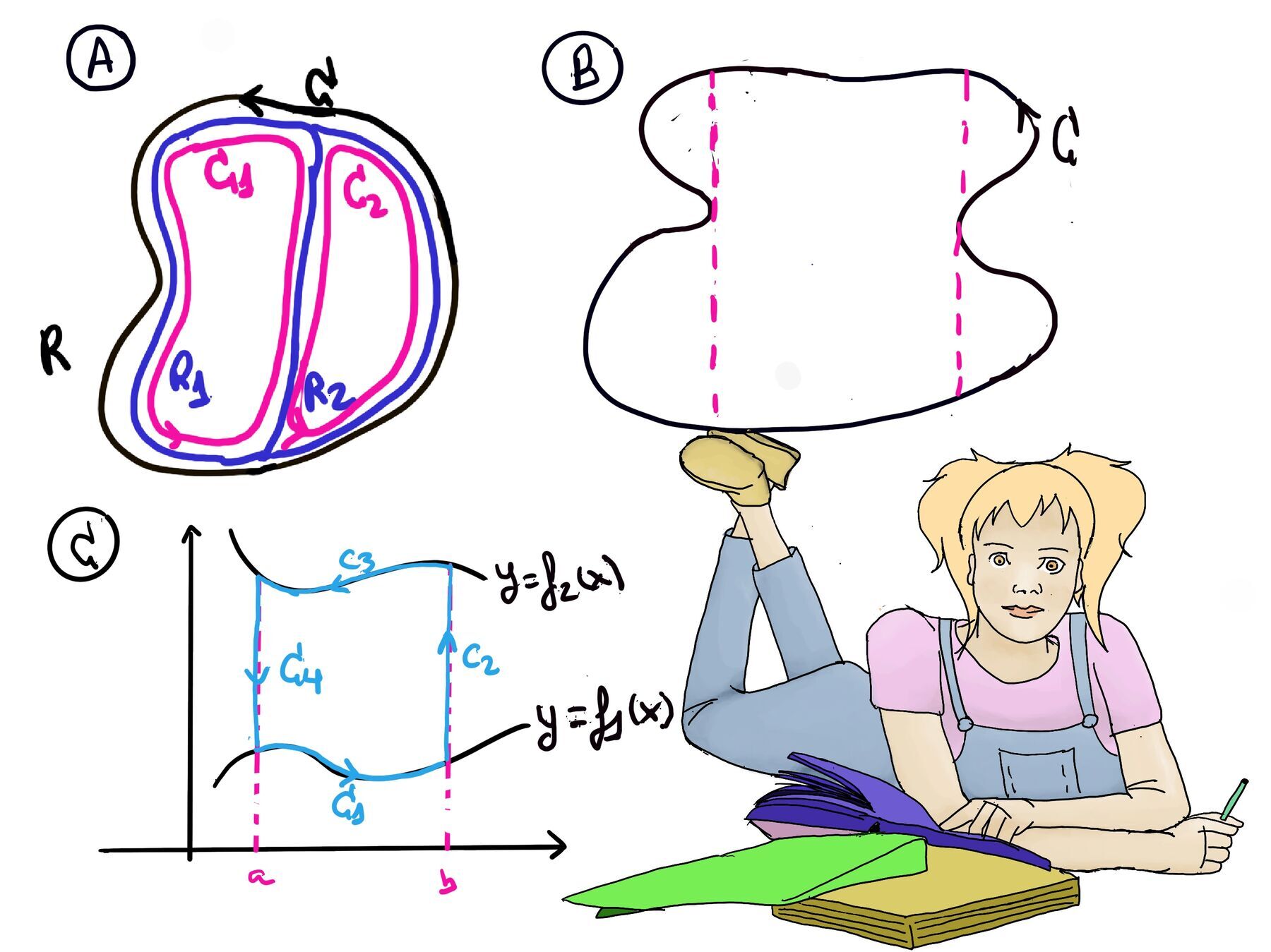
Thus, we have: $\oint_C Mdx =[1] \oint_{C_1} Mdx + \oint_{C_2} Mdx = \iint_{R_1} -M_ydA + \iint_{R_2} -M_ydA = \iint_{R} -M_ydA$

Besides, we are going to cut or split the regions in vertically simple regions (often called a Type I region), which are regions bounded between two curves, $y = f_1(x)$ and $y = f_2(x), \forall x: a \lt x \lt b, f_1(x) \lt y \lt f_2(x)$.

Therefore, we only need to prove $\oint_C Mdx = \iint_R -M_ydA$ if R is vertically simple and C is a boundary of R taken counterclockwise.

Proving the Special Case for a Vertically Simple Region

We split the integral into four parts (Figure C). Let’s consider $R$ as a vertically simple region bounded by the curves $y = f_1(x)$ and $y = f_2(x)$ from $x = a$ to $x = b$. The boundary $C$ can be divided into four segments:

1. Bottom curve ($C_1$): Moving from $a$ to $b$ along $y = f_1(x)$.
   $\oint_{C_1} Mdx =$[Notice that $M = M(x, y), y = f_1(x), a \leq x \leq b$] = $\int_{a}^{b} M(x, f_1(x))dx$

2. Right vertical line ($C_2$): Moving upward at $x = b$. Because $x$ is constant, $dx = 0$. Therefore, this integral evaluates to $0$.

3. Top curve ($C_3$): Moving backward from $b$ to $a$ along $y = f_2(x)$.
   $\oint_{C_3} Mdx =$ [$y = f_2(x), b \leq x \leq a$] = $\int_{b}^{a} M(x, f_2(x))dx = -\int_{a}^{b} M(x, f_2(x))dx$

4. Left vertical line ($C_4$): Moving downward at $x = a$. Again, $x$ is constant, so $dx = 0$. This integral evaluates to $0$.

Putting all together, $\oint_C Mdx = \oint_{C_1} Mdx + \oint_{C_2} Mdx + \oint_{C_3} Mdx + \oint_{C_4} Mdx = \int_{a}^{b} M(x, f_1(x))dx -\int_{a}^{b} M(x, f_2(x))dx = \int_{a}^{b} [M(x, f_1(x))-M(x, f_2(x))]dx$

On the other side of the equation, $\iint_{R} -M_ydA = -\int_{a}^{b}(\int_{f_1(x)}^{f_2(x)} \frac{\partial M}{\partial y}dy)dx$

By the Fundamental Theorem of Calculus, integrating a partial derivative with respect to $y$ just gives us the original function back, evaluated at the bounds: $\int_{f_1(x)}^{f_2(x)} \frac{\partial M}{\partial y}dy = \Big[ M(x,y) \Big]_{y=f_1(x)}^{y=f_2(x)} \, dx$
$-\int_{a}^{b}(\int_{f_1(x)}^{f_2(x)} \frac{\partial M}{\partial y}dy)dx = \int_a^b \Big( -M(x, f_2(x)) - (-M(x, f_1(x))) \Big) dx$

Therefore: $\iint_{R} -M_ydA = -\int_{a}^{b}(\int_{f_1(x)}^{f_2(x)} \frac{\partial M}{\partial y}dy)dx = \int_{a}^{b} [M(x, f_1(x))-M(x, f_2(x))]dx$. The line integral and the double integral yield the exact same result! We have proven that: $\oint_C Mdx = \iint_R -M_ydA$ ∎

Completing the Proof: By using a horizontally simple region (Type II), we can use the exact same logic to prove that $\oint_C Ndy = \iint_R N_x dA$. Adding both halves together gives us the complete Green’s Theorem. Furthermore, any complex shape can be sliced into smaller Type I and Type II regions. Since the interior “cuts” are traversed in opposite directions by adjacent regions, they cancel out, extending our proof to almost any conceivable 2D shape.

Calculate the area of a region

The area of a region R in the plane can be calculated using a double integral over that region. Mathematically, the area is expressed as: $Area(R) = \iint_{R} dA$. Here, $dA$ represents a differential element of area in the region $R$.

However, we can also use Green’s Theorem to find the area of $R$ by converting a double integral over $R$ into a line integral around the boundary $C$ of $R$.

Green’s Theorem states that for a positively oriented, simple, closed curve $C$ enclosing a region $R$: $\oint_{C} Mdx + Ndy = \iint_R (\frac{\partial N}{\partial x}-\frac{\partial M}{\partial y})dA$.

To calculate the area of $R$, we want the double integral on the right-hand side of Green’s Theorem to simply become the area $Area(R) = \iint_{R} dA$. This requires that the expression inside the double integral, $\frac{\partial N}{\partial x}-\frac{\partial M}{\partial y}$, equals 1.

There are several ways to define $M$ and $N$ to obtain this.

• $N = x, M = 0$, then $\oint_{C} Mdx + Ndy = \oint_{C} xdy = \iint_R (\frac{\partial N}{\partial x}-\frac{\partial M}{\partial y})dA = \iint_R(1-0)dA = \iint_R dA = Area(R).$
• $N = 0, M = -y$, then $\oint_{C} Mdx + Ndy = \oint_{C} -ydx =\iint_R (\frac{\partial N}{\partial x}-\frac{\partial M}{\partial y})dA = \iint_R(0-(-1))dA = \iint_R dA = Area(R).$
• Finally, combining the last two options: $N = x, M = -y$, then $\frac{1}{2}\oint_{C} Mdx + Ndy = \frac{1}{2}\oint_{C} xdy-ydx =\frac{1}{2}\iint_R (\frac{\partial N}{\partial x}-\frac{\partial M}{\partial y})dA = \frac{1}{2}\iint_R(1-(-1))dA = \iint_R dA = area(R).$

Example: Area of an Ellipse (Refer to Figure iii for a visual representation and aid in understanding it).

Use a line integral to find the area enclosed by $\frac{x^2}{a^2}+\frac{y^2}{b^2} = 1$.

To apply Green’s Theorem, we parametrize the ellipse using: $x = a\cos(t), y = b\sin(t), 0 \leq t \leq 2\pi$. The differentials are: $ dx = -a \sin(t)dt, dy = b \cos(t)dt$. Bounds: $0 \le t \le 2\pi$.

Using the third option, $M = -y, N = x$, the area enclosed by the ellipse can be computed as: $Area(R)= \frac{1}{2}\oint_{C} xdy-ydx$.

Substitute our parameterizations: $Area(R) = \frac{1}{2}\int_{0}^{2\pi} (a\cos(t))(b\cos(t)dt)-(b\sin(t))(-a\sin(t)dt) =[\text{Simplifying}] \frac{1}{2}\int_{0}^{2\pi}(ab\cos^2(t)+ab\sin^2(t))dt$.

Factor out $ab$: $= \frac{1}{2} \int_0^{2\pi} ab(\cos^2(t) + \sin^2(t)) \, dt$

Because $cos^2(t)+sin^2(t)=1$, the integrand collapses beautifully: $\frac{1}{2}\int_{0}^{2\pi} abdt = \frac{1}{2}abt\bigg|_{0}^{2\pi} = πab$. The area of an ellipse is $\pi a b$. As a bonus, if this were a circle where the radii are equal ($a = b = r$), the formula naturally simplifies to the familiar $Area = \pi r^2$.

Bibliography

1. NPTEL-NOC IITM, Introduction to Galois Theory.
2. Algebra, Second Edition, by Michael Artin.
3. LibreTexts, Calculus. Abstract and Geometric Algebra, Abstract Algebra: Theory and Applications (Judson).
4. Field and Galois Theory, by Patrick Morandi. Springer.
5. Michael Penn, Andrew Misseldine, blackpenredpen, and MathMajor, YouTube’s channels.
6. Contemporary Abstract Algebra, Joseph, A. Gallian.
7. MIT OpenCourseWare, 18.01 Single Variable Calculus, Fall 2007 and 18.02 Multivariable Calculus, Fall 2007, YouTube.
8. Calculus Early Transcendentals: Differential & Multi-Variable Calculus for Social Sciences.