
|
 |

|
|
|
|
|
|
Success is not final, failure is not fatal: It is the courage to continue that counts, Winston Churchill
We shall go on to the end. We shall fight in France, we shall fight on the seas and oceans, we shall fight with growing confidence and growing strength in the air, we shall defend our island, whatever the cost may be. We shall fight on the beaches, we shall fight on the landing grounds, we shall fight in the fields and in the streets, we shall fight in the hills; we shall never surrender, Winston Churchill
A vector field is an assignment of a vector $\vec{F}$ to each point $(x, y)$ in a space.
In two dimensions, this is written as $\vec{F}(x,y) = M(x,y)\mathbf{\hat{i}} + N(x,y)\mathbf{\hat{j}}$. A vector field on a plane can be visualized as a collection of arrows, each attached to a point on the plane, representing vectors with specific magnitudes and directions. Examples include fluid velocity fields, gravitational fields, and electromagnetic fields.
When a vector field represents a force, we often want to calculate the work done by that force as an object moves through it. Work is the energy transferred when a force displaces an object along a path. We calculate this using a line integral along a curve $C$: $\boxed{W = \int_{C} \vec{F} \cdot d\vec{r} = \int_{C} M dx + N dy = \int_{C} \vec{F} \cdot \mathbf{\hat{T}} ds}$ where $\mathbf{\hat{T}}$ is the unit tangent vector to the path $C$.
A vector field $\vec{F}$ is conservative if there exists a scalar function $f$ such that $\vec{F} = \nabla f$. In this case, $\vec{F}$ is simply the gradient of $f$. This scalar function $f$ is known as the potential function associated with the vector field.
Visual Intuition: Imagine a topographical map of a mountain. The altitude at any given coordinate is a scalar function $f(x,y)$. The gradient $\nabla f$ represents the direction of steepest ascent. A vector field is conservative if it perfectly describes the “slope” of some underlying, continuous topological surface.
This leads directly to the Fundamental Theorem of Line Integrals. If $\vec{F}$ is a conservative vector field in a simply connected region, and $f$ is its potential function, then: $\boxed{\int_{C} \vec{F} \cdot d\vec{r} = \int_{C} \nabla f \cdot d\vec{r} = f(P_1) - f(P_0)}$ where $P_0$ and $P_1$ are the initial and final points of the curve $C$.

Conservative force. The line integral of the field around any closed loop $C$ is exactly zero: $\oint_{C} \vec{F} \cdot d\vec{r} = 0$.
In physics, this means moving an object in a circle yields zero net energy change (zero work).
Path independence. The integral between two points is the same, regardless of the trajectory taken. $\int_{C_1} \vec{F} \cdot d\vec{r} = \int_{C_2} \vec{F} \cdot d\vec{r}$ as long as $C_1$ and $C_2$ share the same start and end points.
In physics, the work done by the force in moving an object from one point to another is the same, regardless of the path taken between the two points.
Gradient Field. A vector field $\vec{F}$ is a gradient field if it can be expressed as the gradient of a scalar potential function $f$. In mathematical terms, this means $\vec{F} = \nabla f$, where $f$ is a scalar function and the vector field $\vec{F}$ has components $\vec{F} = \langle M, N \rangle = \langle \frac{\partial f}{\partial x}, \frac{\partial f}{\partial y} \rangle = \langle f_x, f_y \rangle$. Here, $f$ is the potential function associated with the vector field $\vec{F}$.
The lineal integral of $\vec{F}$ along a path $C$ measures the circulation or flow (work if $\vec{F}$ is a force field) done by the vector field in moving an object along the path C. If $\vec{F}$ is a gradient field, then: $\int_{C} \vec{F} \cdot d\vec{r} = f(P_1)-f(P_0).$
Exact differential. In the context of differential forms, a differential expression $Mdx + Ndy$ is called an exact differential if there exist a scalar function $f(x, y)$ such that $df = \frac{\partial f}{\partial x}dx+\frac{\partial f}{\partial y}dy = Mdx + Ndy$. This implies that the vector field $\vec{F} = \langle M, N \rangle$ is conservative, and there exists a potential function f such that $\vec{F} = \nabla f$.
If a differential is exact, then the line integral of $\vec{F}$ over any path C can be evaluated by simply finding the difference in the potential function values at the endpoints of the path.
These four properties —conservative force, path independence, gradient field, and exact differential— are different perspectives of the same fundamental concept: the conservativeness of a vector field.
Finding a potential function can be tedious, so we first need a simple test to guarantee that one actually exists.
The criterion for checking whether a vector field $\vec{F}$ is conservative can be summarized as follows: If $\frac{\partial M}{\partial y} = \frac{\partial N}{\partial x}$, and if the functions $M$ and $N$ have continuous first partial derivatives across the entire domain $D$, and the domain $D$ is both open and simply connected, then $\vec{F}$ is a gradient field, meaning it is conservative.
Do not ignore the requirement that the domain must be simply connected (meaning it has no holes). Consider the classic vortex field: $\vec{F} = \left\langle \frac{-y}{x^2+y^2}, \frac{x}{x^2+y^2} \right\rangle$
If you test the partial derivatives, you will find that $\frac{\partial M}{\partial y} = \frac{\partial N}{\partial x} = \frac{y^2-x^2}{(x^2+y^2)^2}$. It seems quite conservative, isn’t it? However, this field is undefined at the origin $(0,0)$. The domain has a “hole.” If you integrate this field along a closed unit circle around the origin, the result is $2\pi$, not $0$. Because the domain is not simply connected, the component test fails, and the field is not conservative.
A vector field $\vec{F}$ is conservative if it can be expressed as the gradient of some scalar potential function $f(x, y)$. In mathematical terms, this means:$\vec{F} = \nabla f = (\frac{\partial f}{\partial x}, \frac{\partial f}{\partial y})$.
To find a potential function for a conservative vector field, we first need to ensure that the vector field is conservative. A vector field $\vec{F}$ is conservative if $\frac{\partial M}{\partial y} = \frac{\partial N}{\partial x}$, and if the functions $M$ and $N$ have continuous first partial derivatives across the entire domain $D$, and the domain $D$ is open and simply connected, then $\vec{F}$ is a gradient field, meaning it is conservative.
For the vector field $\vec{F}= (4x^2+8xy)\vec{i}+(3y^2+4x^2)\vec{j}$, let’s check if F is conservative.
Since these conditions are met, $\vec{F}$ is indeed conservative, meaning there exists a potential function $f(x, y)$ such that $\vec{F} = \nabla f$.
There are two primary methods to find the potential function: via Line Integrals, and via Antiderivatives.
Because the field is path-independent, we can find $f(x_1, y_1)$ by integrating from the origin $(0,0)$ to $(x_1, y_1)$ along the easiest possible path: moving strictly along the axes (see Figure F.a in the image below).
Assuming our curve $C$ starts at the origin $(0,0)$ and ends at $(x_1, y_1)$: $\int_{C} \vec{F} \cdot d\vec{r} = f(x_1, y_1) - f(0, 0)$.
To find the value of the potential function at the endpoint $f(x_1, y_1)$, we simply use algebra to isolate it: $f(x_1, y_1) = \int_{C} \vec{F} \cdot d\vec{r} + f(0, 0)$ where $f(0, 0)$ is an arbitrary constant.
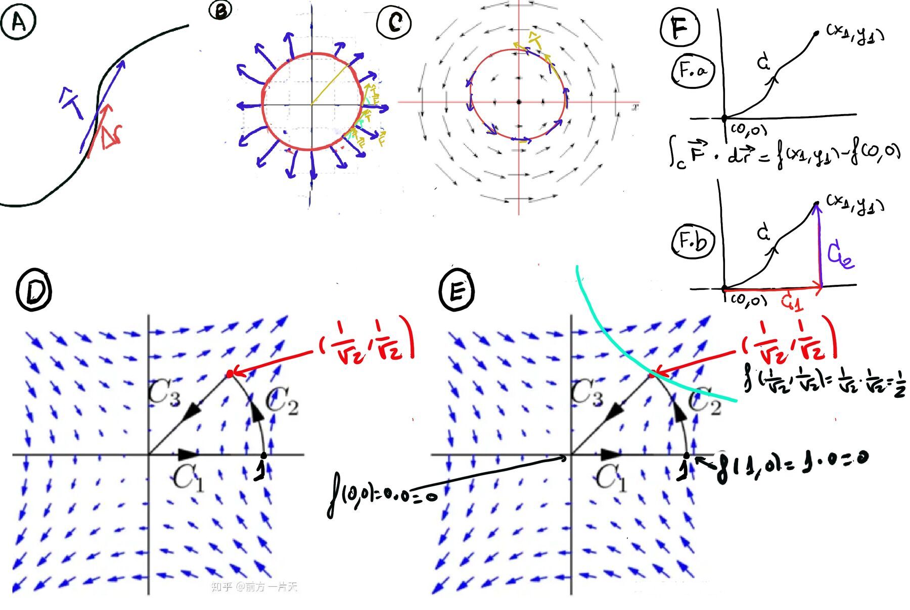
To simplify the calculation, we break the path $C$ into two segments:
Compute the line integral along $C$, $\vec{F}=\langle 4x^2+8xy, 3y^2+4x^2 \rangle$, we have: $\int_{C} \vec{F}\cdot d\vec{r} = \int_{C} (4x^2+8xy)dx + (3y^2+4x^2)dy$
This can be broken down as: $\int_{C_1} (4x^2+8xy)dx + (3y^2+4x^2)dy + \int_{C_2} (4x^2+8xy)dx + (3y^2+4x^2)dy$
$\int_{C_1} (4x^2+8xy)dx + (3y^2+4x^2)dy$ = [x varies from $0$ to $x_1$, $y = 0 \implies dy = 0$] $\int_{0}^{x_1} 4x^2dx = \frac{4}{3}x^3\bigg|_{0}^{x_1} = \frac{4}{3}x_1^3$
$\int_{C_2} (4x^2+8xy)dx + (3y^2+4x^2)dy$ = [y varies from $0$ to $y_1, x = x_1 \implies dx = 0$] $\int_{0}^{y_1} (3y^2+4x_1^2)dy = (y^3+4x_1^2y)\bigg|_{0}^{y_1} = y_1^3+4x_1^2y_1$
Combine the results: $f(x_1, y_1) = \int_{C} \vec{F}\cdot d\vec{r} + f(0, 0) \implies f(x_1, y_1) = \int_{C} \vec{F} \cdot d\vec{r} + c ↭ f(x_1, y_1) = \frac{4}{3}x_1^3 + y_1^3+4x_1^2y_1 + c.$ Therefore, generalizing for any $(x, y)$, $f(x, y) = \int_{C} \vec{F}\cdot d\vec{r} + c = \frac{4}{3}x^3 + y^3+4x^2y + c$ where $c$ is a constant.
For the same vector field, we know that $\vec{F} = \nabla f$ where $F = \langle M, N \rangle = \langle\frac{\partial f}{\partial x}, \frac{\partial f}{\partial y}\rangle = \langle f_x, f_y \rangle$ where $f_x = 4x^2 +8xy$ (i), $f_y = 3y^2 +4x^2$ (ii).
Starting with the partial derivative $f_x (i)$, we integrate with respect to x: $f(x, y) = \int (4x^2+8xy)dx = \frac{4}{3}x^3+4x^2y+g(y)$. Here, $g(y)$ is a function of y that acts as the “constant” of integration when integrating with respect to x (it treats all $y$ terms as constants).
To determine $g(y)$, we differentiate f with respect to y and match it with the given expression for $f_y$:
Differentiate $f$ with respect to $y$: $f_y = 4x^2 + g'(y)$.
Matching this with (ii) $f_y = 3y^2 +4x^2$, we get: $4x^2 + g'(y) = 3y^2 +4x^2 \implies g'(y) = 3y^2$
Integrate $g′(y)$ with respect to $y$: $g(y) = \int g'(y)dy = \int 3y^2dy = y^3 + c$ and $c$ is a real constant.
Substituting $g(y) = y^3 +c$ back into our equation for f(x, y), we get: $f(x, y) = \frac{4}{3}x^3+4x^2y+g(y) = \frac{4}{3}x^3+4x^2y+ y^3 +c$
Step 1. Check if $\vec{F}$ is a conservative vector field.
To find a potential function for a conservative vector field, we first need to ensure that the vector field is conservative. A vector field $\vec{F}$ is conservative if $\frac{\partial M}{\partial y} = \frac{\partial N}{\partial x}$, and if the functions $M$ and $N$ have continuous first partial derivatives across the entire domain $D$, and the domain $D$ is open and simply connected, then $\vec{F}$ is a gradient field, meaning it is conservative.
Given: M = $ye^x+sin(y)$, N = $e^x+xcos(y)$
Since these conditions are met, $\vec{F}$ is indeed conservative, meaning there exists a potential function $f(x, y)$ such that $\vec{F} = \nabla f$.
Step 2. Finding the potential function f using Antiderivatives
For the same vector field, we know that $\vec{F} = \nabla f$ where $F = \langle M, N\rangle = \langle\frac{\partial f}{\partial x}, \frac{\partial f}{\partial y}\rangle = \langle f_x, f_y \rangle$ where $f_x(x, y) = ye^x +\sin(y)$ (i), $f_y(x, y) = e^x +x\cos(y)$ (ii).
From (i), we integrate with respect to x: $f(x, y) = \int (ye^x + \sin(y))dx = ye^x + x\sin(y) +g(y)$ where $g(y)$ is a function of y (acting as the constant of integration with respect to x, but not necessarily for y), i.e., the integration constant can depend on y.
To determine $g(y)$, we differentiate f with respect to y: $f_y(x, y) = \frac{\partial f}{\partial y} = \frac{\partial}{\partial y}(ye^x + x\sin(y)+g(y)) = e^x + xcos(y) + g'(y)$. Matching this with (ii) we get: $f_y(x, y) = e^x+xcos(y)$. Thus, $e^x +x\cos(y) = e^x+cos(y)+g'(y) \implies g'(y) =0$
Integrating $g′(y)$ with respect to $y: g(y) = \int 0dy = c$ and $c$ is a real constant.
Therefore, the potential function $f$ is: $f(x, y) = ye^x +x\sin(y) + c$. This function represents the scalar potential associated with the conservative vector field $\vec{F}$.
For a 3D vector field $\vec{F}(x, y, z) = P\mathbf{\hat{i}} + Q\mathbf{\hat{j}} + R\mathbf{\hat{k}}$, checking mixed partials requires testing three pairs. The formal mathematical tool for this is the Curl operator.A 3D vector field over a simply connected domain is conservative if and only if its curl is zero: $\boxed{\nabla \times \vec{F} = \vec{0}}$.
Given: $P = yz, Q = xz, R = (xy+2z)$.
Step 1: Check if $\vec{F}$ is conservative. The vector field is in three dimensions, so we will follow a similar process as before but adapted for three variables.
Since these conditions are met, $\vec{F}$ is indeed conservative, meaning there exists a potential function $f(x, y, z)$ such that $\vec{F} = \nabla f$.
Step 2: Find the Potential Function $f(x, y, z)$
We have $f_x(x, y, z) = yz$ (i), $f_y(x, y, z) = xz$ (ii), $f_z(x, y, z) = xy + 2z$ (iii).
From (i) integrate $f_x = yz$ with respect to $x$: $f(x, y, z) = \int (yz)dx = yzx + g(y, z)$ where $g(y, z)$ is a function of y and z because it acts as the “constant” of integration with respect to x, but not necessarily for y and z.
To determine g(y), we differentiate f with respect to y and z:
Differentiate with Respect to y: $f_y(x, y, z) = \frac{\partial}{\partial y}(yzx + g(y, z)) = xz + g_y(y, z)$. Matching this with (ii), $f_y(x, y, z) = xz$, we get: $xz = xz + g_y(y, z) \implies g_y(y, z) = 0$. Integrating $g_y(y, z)$ with respect to y, we get, $g(y, z) = h(z)$, so $g(y, z)$ is a function of z alone.
Differentiate with Respect to z: $f_z(x, y, z) = \frac{\partial}{\partial z}(yzx + h(z)) = yx + h'(z)$. Matching this with (iii), $f_z(x, y, z) = xy + 2z$ we get: $yx + h'(z) = xy + 2z \implies h'(z) = 2z$. Integrating $h(z)$ with respect to $z$, we get, $h(z) = z^2 + k$.
Therefore, the potential function $f(x, y, z) = xyz + g(y, z) = xyz + h(z) = xyz + z^2 + k$.
Step 3. Evaluating the line integral $\int_{C} \vec{F} \cdot d\vec{r}$
The line integral of a conservative vector field $\vec{F}$ over a curve $C$ from point $A$ to point $B$ can be evaluated using the potential function f: $\int_{C} \vec{F}\cdot d\vec{r} = f(B) - f(A)$
Here, $C$ is the line segment from $A = (1, 0, −2)$ to $B = (4, 6, 3)$.
$\int_{C} \vec{F}\cdot d\vec{r} = \int_{C} \nabla f\cdot d\vec{r} = f(4, 6, 3) -f(1, 0, -2) = 4 \cdot 6 \cdot 3 + 3^2 + c -(1\cdot0\cdot(-2)+(-2)^2 + c) = 72 +9 -4 = 81 -4 = 77.$
When calculating the work done by a force field along a curve, the most tedious approach is to manually parameterize the path. Fortunately, if the vector field is conservative, the path taken doesn’t matter. The work done relies entirely on the starting and ending points.
This principle —the Fundamental Theorem of Line Integrals— is the multivariable equivalent of the Fundamental Theorem of Calculus. In physics, this is why the energy required to lift a box to the top shelf is the same whether you lift it straight up or carry it up a ramp.
If a vector field $\vec{F}(x,y) = \langle P(x,y), Q(x,y) \rangle$ is conservative on an open, simply-connected domain, it is the gradient of a scalar potential function $f(x,y)$. That means: $\boxed{\vec{F} = \nabla f = \left\langle \frac{\partial f}{\partial x}, \frac{\partial f}{\partial y} \right\rangle}$
To evaluate the line integral $\int_C \vec{F} \cdot d\vec{r}$, we only need to find this potential function $f$ and evaluate it at the endpoints: $\boxed{\int_C \vec{F} \cdot d\vec{r} = f(B) - f(A)}$
Let’s explore three problems that require us to prove a field is conservative, find its potential function, and evaluate the work done.
Step 0: Check if $\vec{F}$ is conservative.
Since all the conditions are met, $\vec{F}$ is indeed a conservative vector field.
Step 1. Calculate the potential function
Because $\vec{F} = \nabla f$, we know that $f_x = P$ and $f_y = Q$.
$f_x = y\cos(x)+y^2$. Let’s integrate with respect to x, $f = \int f_xdx = \int y\cos(x)+y^2dx = y\sin(x) + y^2x + g(y)$. Here, $g(y)$ is a function of y that acts as the “constant” of integration when integrating with respect to x.
Similarly, $f_y = \sin(x) + 2xy -2y$. Let’s derivative f with respect to y, $f_y = \frac{\partial f}{\partial y} = \frac{\partial}{\partial y}(y\sin(x) + y^2x + g(y)) = \sin(x) +2yx +g'(y)$
Setting this equal to the original $Q(x, y)$: $\sin(x) +2yx +g'(y) = \sin(x) + 2xy -2y \implies g'(y) = -2y$.
Let’s integrate g with respect to y, $g = \int -2ydy = -y^2 + k$.
Combining these results together: $f = y\sin(x) + y^2x + g(y)= y\sin(x) + y^2x + -y^2 + k$
Step 2. Evaluating work or the line integral $\int_{C} \vec{F} \cdot d\vec{r}$
The line integral of a conservative vector field $\vec{F}$ over a curve C from point A to point B can be evaluated using the potential function f: $Work = \int_{C} \vec{F} \cdot d\vec{r} = f(\frac{\pi}{2}, -1) - f(-\pi, 2)$.
Evaluate at the endpoint $f(\frac{\pi}{2}, -1)$: $f(\frac{\pi}{2}, -1) = (-1)sin(\frac{\pi}{2})+\frac{\pi}{2}(-1)^2-(-1)^2+k = -1 + \frac{\pi}{2}-1+ k = \frac{\pi}{2}-2+k.$
Evaluate at the starting point $f(-\pi, 2)$: $f(-\pi, 2) = 2\sin(-\pi) +2^2(-\pi)-4+k = 0-4\pi-4+C$
Work = $\int_{C} \vec{F}\cdot d\vec{r} = f(\frac{\pi}{2}, -1) - f(-\pi, 2) = \frac{\pi}{2}-2+k +4\pi+4-k = \frac{9\pi}{2}+2$
Step 0: Check if $\vec{F}$ is conservative.
Since all the conditions are met, $\vec{F}$ is indeed a conservative vector field.
Step 1. Calculate the potential function
$f_x = e^{2y}$. Let’s integrate with respect to x, $f = \int f_xdx = \int e^{2y}dx = e^{2y}x + g(y)$. Here, $g(y)$ is a function of y that acts as the “constant” of integration when integrating with respect to x.
Similarly $f_y = 1 +2xe^{2y}$. Let’s integrate with respect to y, $f = \int f_ydy = \int 1 +2xe^{2y}dy = y + xe^{2y} + h(x)$.
Combining these results together: $g(y) = y, h(x) = 0, f(x, y) = y + xe^{2y}$
Step 2. Evaluating work or the line integral $\int_{C} \vec{F} \cdot d\vec{r}$
The line integral of a conservative vector field $\vec{F}$ over a curve C from point A to point B can be evaluated using the potential function f: $Work = \int_{C} \vec{F} \cdot d\vec{r}$
Note: The constant $C$ cancels out during subtraction, so we can omit it during evaluation.
First, we must find the Cartesian coordinates for points $A$ and $B$ by evaluating $\vec{r}(t)$ at $t=0$ and $t=1$.
Starting Point $A$ ($t=0$): $\vec{r}(0) = \langle e^0, 1 + 0 \rangle = (1, 1)$.
Endpoint $B$ ($t=1$): $\vec{r}(1) = \langle e^1, 1 + 1 \rangle = (e, 2)$.
Now, apply the Fundamental Theorem of Line Integrals: $\text{Work} = f(e, 2) - f(1, 1)$
$f(e, 2) = (e)(e^{2(2)}) + 2 = e^5 + 2$, $f(1, 1) = (1)(e^{2(1)}) + 1 = e^2 + 1$
$\text{Work} = (e^5 + 2) - (e^2 + 1) = e^5 - e^2 + 1$
Step 1: Frame the Vector Field
The given integral can be interpreted as a line integral of a vector field. We define the vector field $\vec{F}(x, y)$ as $\vec{F}(x, y) = \langle M, N \rangle = M\vec{i}+ N\vec{j} = 2xe^{-y}\vec{i}+ (2y-x^2e^{-y})\vec{j}$
Step 2: Prove Path Independence
We can confirm that $\vec{F}$ is defined everywhere in $\mathbb{R}^2$. Because the components $M(x, y)$ and $N(x,y)$ involve polynomials and exponential functions, they possess continuous first partial derivatives. Besides, $\mathbb{R}^2$ is both open and simply-connected domain.
To determine if the vector field $\vec{F} = \langle M, N\rangle$ is conservative, we check if it satisfies the condition $N_x = M_y$. This means that the mixed partial derivatives of the potential function must be equal.
Given: $M = 2xe^{-y}, N = 2y-x^2e^{-y}$. Calculate the partial derivatives:
$\frac{\partial M}{\partial y} = \frac{\partial}{\partial y}(2xe^{-y}) = -2xe^{-y}, \frac{\partial N}{\partial x} = \frac{\partial}{\partial x}(2y-x^2e^{-y}) = -2xe^{-y}$. Because $N_x = M_y$, $\vec{F}$ is a conservative vector field, and therefore, the line integral over any path from $(1, 0)$ to $(2, 1)$ is path-independence.
Step 3. Calculate the potential function $f(x, y)$
For the same vector field, we know that $\vec{F} = \nabla f$ where F = $\langle M, N\rangle = \langle\frac{\partial f}{\partial x}, \frac{\partial f}{\partial y}\rangle = \langle f_x, f_y \rangle$
Given: $M = f_x(x, y) = 2xe^{-y}$ (i), $N = f_y(x, y) = 2y-x^2e^{-y}$ (ii)
$M = f_x(x, y) = 2xe^{-y}$. To find $f(x, y)$, we integrate $f_x$ with respect to x: $f(x, y) = \int f_x(x, y)dx = \int 2xe^{-y}dx = 2e^{-y}\int xdx = 2e^{-y}\frac{x^2}{2}+g(y) = x^2e^{-y} + g(y)$
Here, $g(y)$ is a function of y acting as the constant of integration with respect to x.
To determine $g(y)$, we differentiate $f(x, y) = x^2e^{-y} + g(y)$ with respect to y:
$f_y(x, y) = \frac{\partial}{\partial y}(x^2e^{-y} + g(y)) = -x^2e^{-y}+g'(y)$
Matching this with (ii) $f_y(x, y) = 2y-x^2e^{-y}$, we get $2y-x^2e^{-y} = -x^2e^{-y}+g'(y) \implies g'(y)=2y$
Let’s integrate with respect to y, $g(y)= y^2 +c$
Therefore, the potential function f is: $f(x, y) = x^2e^{-y} + g(y) = x^2e^{-y} + y^2 +c$
Step 4. Evaluating the line integral $\int_{C} \vec{F} \cdot d\vec{r}$
The line integral of a conservative vector field $\vec{F}$ over a curve C from point A to point B can be evaluated using the potential function f: $\int_{C} \vec{F} \cdot d\vec{r} = f(B) - f(A)$ Here, C is any path from $(1, 0)$ to $(2, 1)$.
$\int_{C} \vec{F}\cdot d\vec{r} = \int_{C} \nabla f\cdot d\vec{r} = f(2, 1)-f(1, 0) = (4e^{-1} + 1^2 +c)-(1^2e^{0} + 0^2 +c) = \frac{4}{e}+1+c-1-c = \frac{4}{e}.$

JustToThePoint Copyright © 2011 - 2026 Anawim. ALL RIGHTS RESERVED. Bilingual e-books, articles, and videos to help your child and your entire family succeed, develop a healthy lifestyle, and have a lot of fun. Social Issues, Join us.
This website uses cookies to improve your navigation experience.
By continuing, you are consenting to our
use of cookies, in accordance with our Cookies Policy and
Website Terms and Conditions of use.