Deformation of contours

The excitement of learning separates youth from old age. As long as you’re learning, you’re not old, Rosalyn S.Yalow

Introduction

A complex function $f(z)$ maps $z = x + iy \in \mathbb{C}$ to another complex number. For example: $f(z) = z^2 = (x + iy)^2 = x^2 - y^2 + 2ixy, f(z) = \frac{1}{z}, f(z) = \sqrt{z^2 + 7}$.

A contour is a continuous, piecewise-smooth curve defined parametrically as: $z(t) = x(t) + iy(t), \quad a \leq t \leq b$.

Definition (Smooth Contour Integral). Let ᵞ be a smooth contour (a continuously differentiable path in the complex plane), $\gamma: [a, b] \to \mathbb{C}$. Let $f: \gamma^* \to \mathbb{C}$ be a continuous complex-valued function defined on the trace $\gamma^*$ of the contour (i.e. along the image of $\gamma$). Then, the contour integral of f along $\gamma$ is defined as $\int_{\gamma} f(z)dz := \int_{a}^{b} f(\gamma(t)) \gamma^{'}(t)dt$.

Properties

• Cauchy Integral Formula. If a function f is analytic in a simply connected domain D and γ is a simply closed contour (positive orientated) in D. Then, for any point $z_0$ inside γ we have $f(z_0) = \frac{1}{2\pi i}\cdot \int_{\gamma} \frac{f(z)}{z-z_0}dz$ (Figure D).

• The Residue Theorem states that the integral of a function f(z) around a simple (doesn't cross itself), and positively oriented (counter-clockwise) contour γ is equal to 2πi times the sum of the residues of all singularities inside the contour, $\int_{\gamma} f(z)dz = 2\pi i \sum Res(f, z_k)$ where $z_k$ is a reside inside γ. f must be analytic inside the contour γ, except for a finite number of isolated singularities.

1. For a simple pole at a point $z_k$ (i.e., the denominator has a simple root) is calculated using the formula $Res(f, z_k) = \lim_{z \to z_k}(z-z_k)f(z)$.
2. For a pole of order m, $Res(f, z_k) = \frac{1}{(m-1)!}\lim_{z \to z_k} \frac{d^{m-1}}{dz^{m-1}}[(z-z_k)^mf(z)]$

• Proposition. Linearity of the contour integral, $\int_{\gamma} (af(z) + bg(z))dz = a\int_{\gamma} f(z)dz + b\int_{\gamma} g(z)dz$
• Proposition. Properties of contour integrals under path manipulation. Let γ be a contour, defined by a function $\gamma: [a, b] \to \mathbb{C}$ and let f be a continuous functions $f: \gamma^* \to \mathbb{C}$ defined along the image of ᵞ. Then,

1. Reversal of orientation. $\int_{-\gamma} f(z)dz = -\int_{\gamma} f(z)dz$ where $-\gamma:[a,b] \to \mathbb{C}$ is the reverse of the contour (traversing the same path in the opposite direction) defined by $(- \gamma)(t)=\gamma(a+b-t)$. This property states that reversing the direction of a contour changes or flips the sign of the integral. Intuitively, this is analogous to how reversing the limits of integration in real analysis changes the sign: $\int_a^b f(x)dx = -\int_b^a f(x)dx$. In complex analysis, the orientation of the contour matters because the integral depends on the direction in which we traverse the path.
2. Additivity under subdivision. Suppose a < c < b, let split $\gamma$ into two sub-contours $\gamma_1 = \gamma|_{[a, \gamma_1]} \text{ and } \gamma_2 = \gamma|_{[c, b]}$, then $\int_{\gamma} f(z)dz = \int_{\gamma_1} f(z)dz + \int_{\gamma_2} f(z)dz$. This property states that integrating over the whole contour is the same as integrating over the pieces successively. This is the complex analogue of the additive property of definite integrals: $\int_a^b f(x)dx = \int_a^c f(x)dx + \int_c^b f(x)dx $ for a < c < b.
3. Invariance of Contour Integrals Under Reparameterization. Let $\tilde{\gamma}$ be a contour, defined by a function $\tilde{\gamma}: [c, d] \to \mathbb{C}$. If $\tilde{\gamma}$ is another parameterization of the same oriented path $\gamma$ meaning there exists a one-to-one, continuously differentiable map $\psi: [c,d]\to[a,b]$ with a positive derivative $\psi'(t)>0$ such that $\tilde{\gamma}(t) = \gamma(\psi(t))$, then $\int_{\gamma} f(z)dz = \int_{\tilde{\gamma}} f(z)dz$

• Deformation of Contours. If two contours $\gamma_1$ and $\gamma_2 $ are homotopic (i.e., one can be continuously deformed into the other without crossing any singularities of f) in a domain where f(z) is analytic, then: $\int_{\gamma_1} f(z)dz = \int_{\gamma_2} f(z)dz.$

• Fundamental Theorem of Calculus for Contours. Suppose $\gamma$ is a contour (piecewise smooth path) from a to b, f is defined on a domain D containing $\gamma^*$ (the image of $\gamma$) and admits a primitive (antiderivative) F on D (i.e., $F'(z) = f(z)$), then $\int_{\gamma} f(z)dz = F(\gamma(b)) - F(\gamma(a))$. In particular, if $\gamma$ is a closed contour (i.e., $\gamma(a)=\gamma(b)$), this integral evaluates to zero, $\int_{\gamma} f(z)dz = 0.$

• Estimation Theorem or the Triangle Inequality for Integrals. The triangle inequality for integrals in complex analysis states thatfor any continuous complex function $f:[a,b] \to \mathbb{C}$ on a closed real interval [a,b] (f(t) = u(t) + iv(t), t a real parameter), the following holds: $∣\int_a^b f(t)dt| \leq \int_a^b |f(t)|dt$.

• Estimation Lemma (ML Inequality) for contour integrals. For any continuous complex function $f:[a,b] \to \mathbb{C}$ on a closed real interval [a,b] (f(z) = u(x, y) + iv(x, y)) with f bounded by some constant M along the entire contour, |f(z)| ≤ M for all $z \in \gamma^*$ (the image/trace of the contour in the complex plane), the following holds: $∣\int_\gamma f(z)dz| \leq M \cdot l(\gamma)$ where l(γ) is the arc length of the contour γ given by $\int_a^b |\gamma^{'}(t)|dt = \int_a^b \sqrt{x'(t)^2 + y'(t)^2} \text{ where } \gamma(t) = x(t) + iy(t)$.

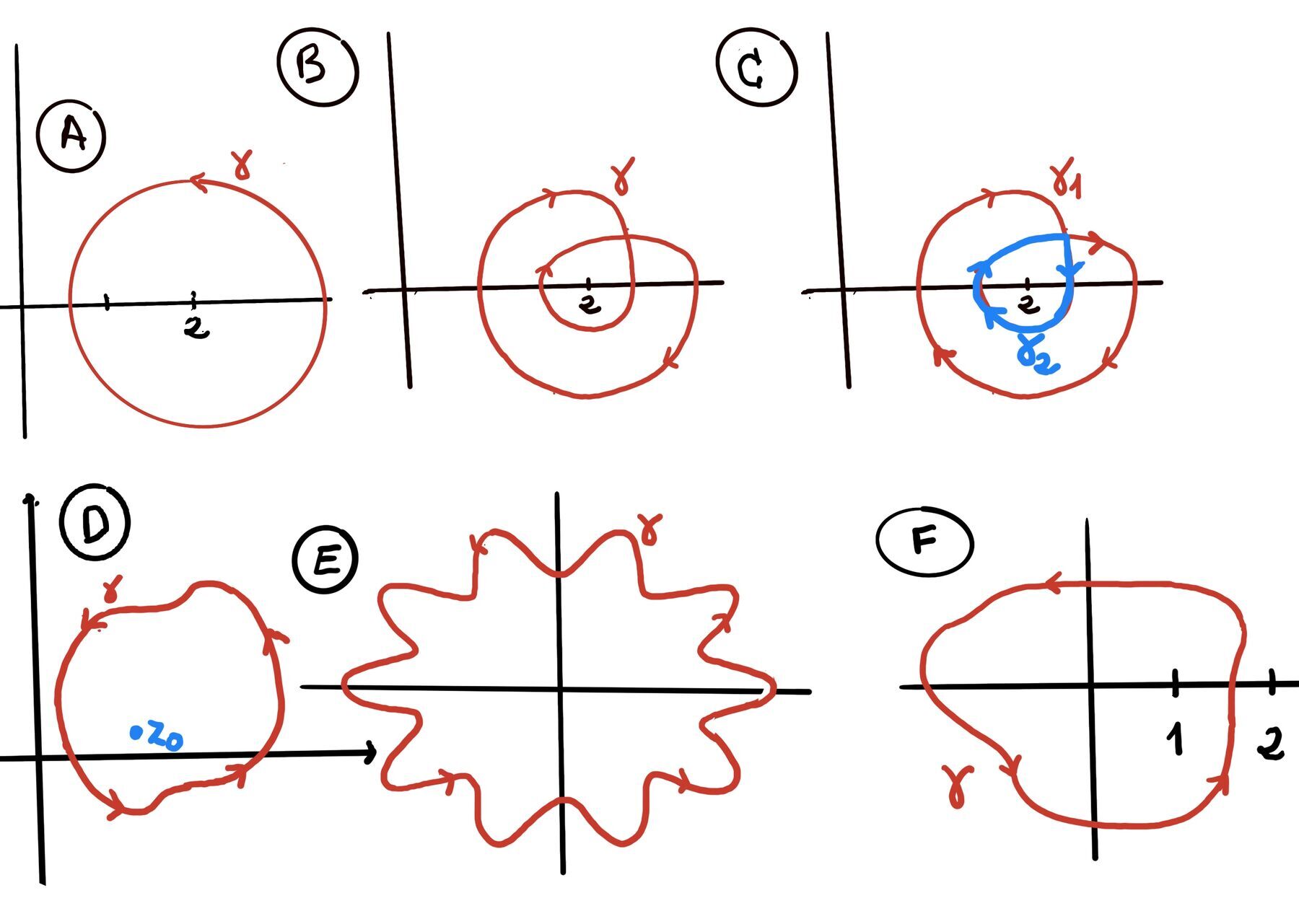
• Jordan’s curve theorem. Any simple closed curve (a continuous loop in the plane that does not intersect itself) separates the plane into two disjoint connected regions: one interior (bounded) and one exterior (unbounded). The curve itself is the boundary of both regions. In other words, it partitions the plane into exactly three disjoint sets:

1. The Curve itself ($\gamma$).
2. The Interior (Int($\gamma$)) is the finite area enclosed by the curve (e.g., if you draw a circle on a piece of paper, the interior region would be everything inside the circle). It is a bounded, simply connected region.
3. The Exterior (Ext($\gamma$)) is the infinite area outside the curve (e.g., using the same circle example, the exterior region would include all points on the paper that are not inside the circle). It is an unbounded region.

• Definition. Let $\gamma: [α, β] → \mathbb{C}$ be a piecewise smooth, closed curve (so γ(α) = γ(β)), the winding number of γ about $z_0$, a complex point not on the curve $z_0$ ∉ γ([α, β]), also known as the index of $z_0$ with respect to γ, is defined as $n(\gamma, z_0) = Ind_{\gamma}(z_0) = \frac{1}{2\pi i} \oint_{\gamma} \frac{dz}{z - z_0} = \frac{1}{2\pi i} \int_{\alpha}^{\beta} \frac{\gamma'(t)}{\gamma(t) - z_0}dt$ (the total number of counterclockwise turns that the object makes around $z_0$).

Cauchy’s Theorem in Complex Analysis

• Cauchy’s theorem (Classical “Green’s theorem” version). Let $\Omega \subset \mathbb{C}$ be an open domain. Suppose f = u + iv is analytic in $\Omega$ and its partial derivatives ( $u_x,u_y,v_x,v_y$) are continuous in $\Omega$. If $\gamma$ is a positively oriented, piecewise-smooth $C^1$, simple closed contour with $\gamma^* \cup \operatorname{Int}(\gamma) \subset \Omega$ (its path and interior both lie inside Ω), then $\oint_{\gamma} f(z)dz = 0.$

• Cauchy’s Theorem (Cauchy–Goursat). This is the more powerful version, as it removes the need for continuous partial derivatives. If f is analytic in an open set containing a simple closed contour γ and its interior $\gamma^*\cup\operatorname{Int}(\gamma)$, then $\oint_{\gamma} f(z)dz = 0$.

• Cauchy’s Theorem for simply connected domains. If a function f is analytic (a function that is complex-differentiable at every point within a domain, i.e., well-behaved and smooth, with no sharp corners, breaks, or singularities like division by zero) throughout a simply simple connected domain D then $\oint_C f(z)dz = 0$ for every closed contour C lying in D.

• General Cauchy Theorem for Multiply Connected Domains. Let $R$ be the multiply connected region (with n holes) inside $C$ but outside of every $C_k$ (each $C_k$ surrounds only one hole in the domain), $R = Int(C) \setminus \bigcup_{k=1}^n \overline{​Int(C_k​)}$​, and let $f(z)$ be analytic on $R$. Now, let $\Gamma$ be any general closed contour (not necessarily simple) that lies entirely in R. This $\Gamma$ can wind around the “holes” (the regions inside each $C_k$) in any way it likes (this is the winding number or index of $\Gamma$ around each hole), the integral over $\Gamma$ is: $\oint_{\Gamma} f(z)dz = \sum_{k=1}^n m_k \oint_{C_k} f(z)dz$.

The Anti-Derivative Theorem

The Anti-Derivative Theorem. Let f be a continuous function on a region G (a region is an open, connected set). Then, the following statements are equivalent:

1. f has an antiderivative F throughout G. This means a function F exists such that F is analytic and F’(z) = f(z) for any z ∈ G.
2. The integral of f over every closed contour $\gamma$ in $G$ is zero: $\oint_\gamma f(z)dz = 0$.
3. The integral of $f$ is path independence. For any two points $a$ and $b$ in $G$, the value of $\oint_\gamma f(z)dz$ is the same (constant) for any contour $\gamma$ in $G$ that starts at a and ends at b.

Deformation of contours

Informal definition. Deformation of contours. Think of a closed rubber band γ₀ lying in a domain D. A loop or closed contour $\gamma_0$ is continuously deformed into the loop $\gamma_1$ in the domain D if you can stretch, shrink, or slide $\gamma_0$ without ever leaving D and without cutting or gluing, until it exactly coincides or matches $\gamma_1$ (same position and orientation), Figure iii.

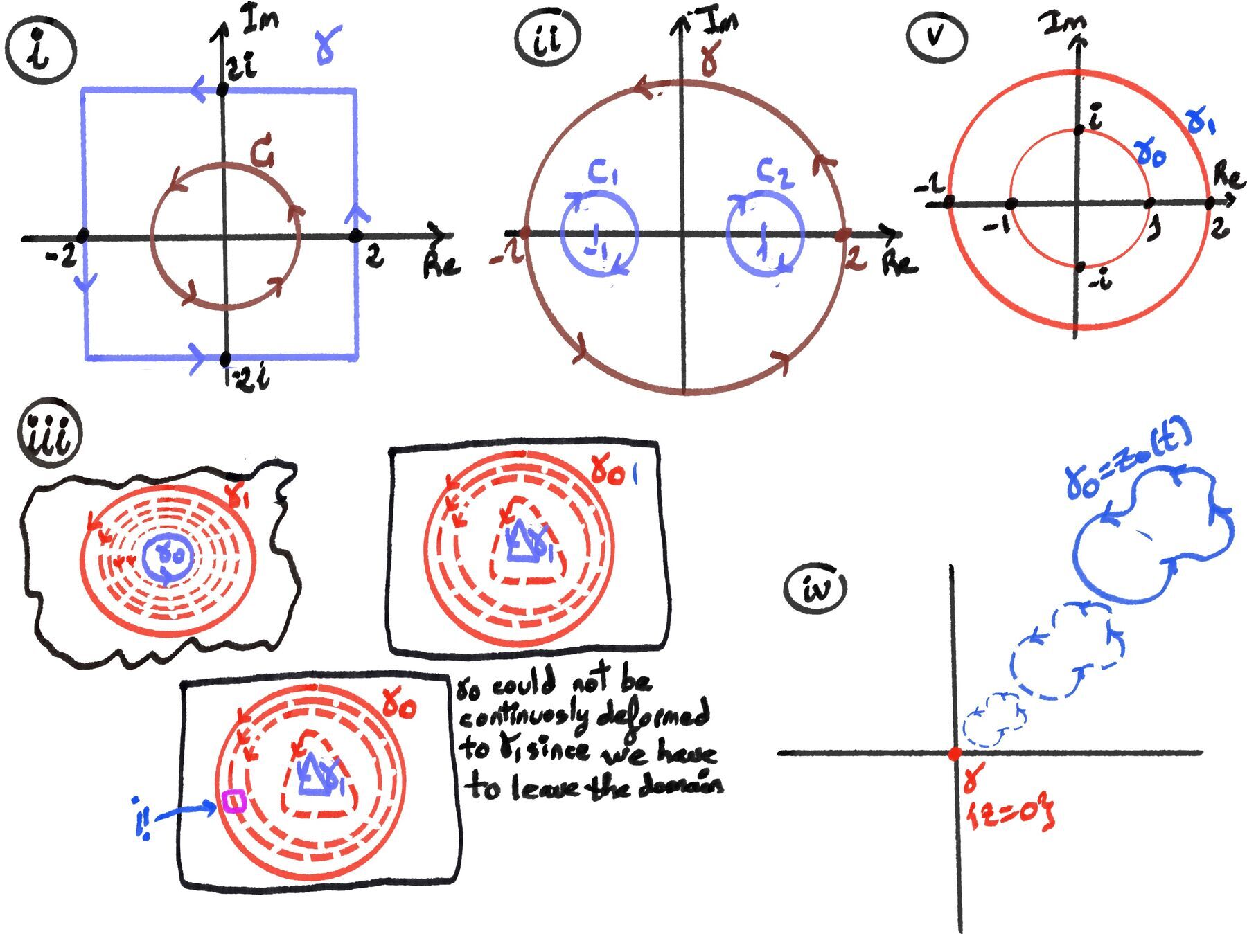
Basically, we need a set (a continuum of loops sufficiently close one to another) $\{ \gamma_s \}, 0 \le s \le 1 = \gamma_0, \gamma_{00\cdots 01}, \cdots, \gamma_{09\cdots 91}, \gamma_1$ where we move from one loop to another by stretching, shrinking, or sliding without ever leaving the domain D.

Formal definition. Deformation of contours. A homotopy (continuous deformation) from a loop (closed contour) $\gamma_0$ to the loop $\gamma_1$, γ₀ ≃ γ₁, in the domain D is a continuos function z: [0, 1] x [0, 1] → D, (s, t) → z(s, t) that satisfies:

• for every fixed s in [0, 1], z(s, t) parametrizes a loop $\gamma_s$ in D, i.e., γₛ(t) := H(s,t)is a closed loop in D, 0 ≤ t ≤ 1.
• γ₀(t) = z(0, t) parametrizes the initial loop $\gamma_0$.
• γ₁(t) = z(1, t) parametrizes the final loop $\gamma_1$.

Examples

• Collapse to a point (shows ℂ is simply connected). Any loop γ₀ in the complex plane can be shrunk to the point contour γ, {z = 0} (Figure iv).

Let γ₀ be parameterized as γ₀ = z₀(t), 0 ≤ t ≤ 1. Consider the function z(s, t) = (1 - z)·z₀(t), 0 ≤ s ≤ 1, 0 ≤ t ≤ 1. z(0, t) = (1 - 0)·z₀(t) = z₀(t). At s = 1 the loop shrinks to the constant loop, z(1, t) = (1 - 1)·z₀(t) ≡ 0.

Any domain D possessing the property that every loop in D can be continuously deformed to a point is called a simply connected domain. Intuitively, a simply connected domain is a domain without “holes”.

• Radial expansion in an annulus. The loop γ₀: z₀(t) = $e^{2\pi i t}$, 0 ≤ t ≤ 1, can be deformed to the loop γ₁: z₀(t) = $2e^{2\pi i t}$, 0 ≤ t ≤ 1 in D = { ½ < |z| < 3 } (Figure v). Consider the function $z(s, t) = (1 + s)e^{2\pi it}, 0 ≤ s ≤ 1, 0 ≤ t ≤ 1; z(0, t) = (1 - 0)·z₀(t) = e^{2\pi it} = z₀(t) ≡ \gamma_0; z(1, t) = (1 + 1)·z₀(t) = 2e^{2\pi it} ≡ \gamma_1$, hence γ₀ ≃ γ₁ in D.
• Impossible deformation (presence of a hole). Let D = ℂ \ {½}. $γ₀(t)=e^{2πit}$ cannot be deformed to a point in D because the winding number around 0 is 1 for every s, while a constant loop has winding number 0. Thus D is not simply connected.

Deformation of Contours Theorem

Deformation of Contours Theorem. If a function f(z) is analytic throughout a region G, and if γ₁ and γ₂ are two simple closed, positively oriented contours that are homotopic in G (meaning $\gamma_1$ can be continuously deformed into $\gamma_2$ entirely within $G$ without crossing any singularities of f), then their contour integrals are equal: $\oint_{\gamma_1} f(z)dz = \oint_{\gamma_2}f(z)dz$.

The integral of an analytic function is invariant under deformation of the contour, provided the deformation doesn’t cross a point where $f(z)$ is not analytic.

Proof.

We define two arbitrary, non-intersecting line segments or cuts $L_1$ and $L_2$. $L_1$ and $L_2$ start on $\gamma_1$ and end on $\gamma_2$. They both divide the space between $\gamma_1$ and $\gamma_2$ and also divide the original contours:

• $\gamma_1$ is split into $\gamma_1^*$ (path between $L_1$ and $L_2$) and $\gamma_1^{**}$ (the remainder).
• $\gamma_2$ is split into $\gamma_2^*$ (path between $L_1$ and $L_2$) and $\gamma_2^{**}$ (the remainder).
  Note that the original contours are traversed positively (counter-clockwise).

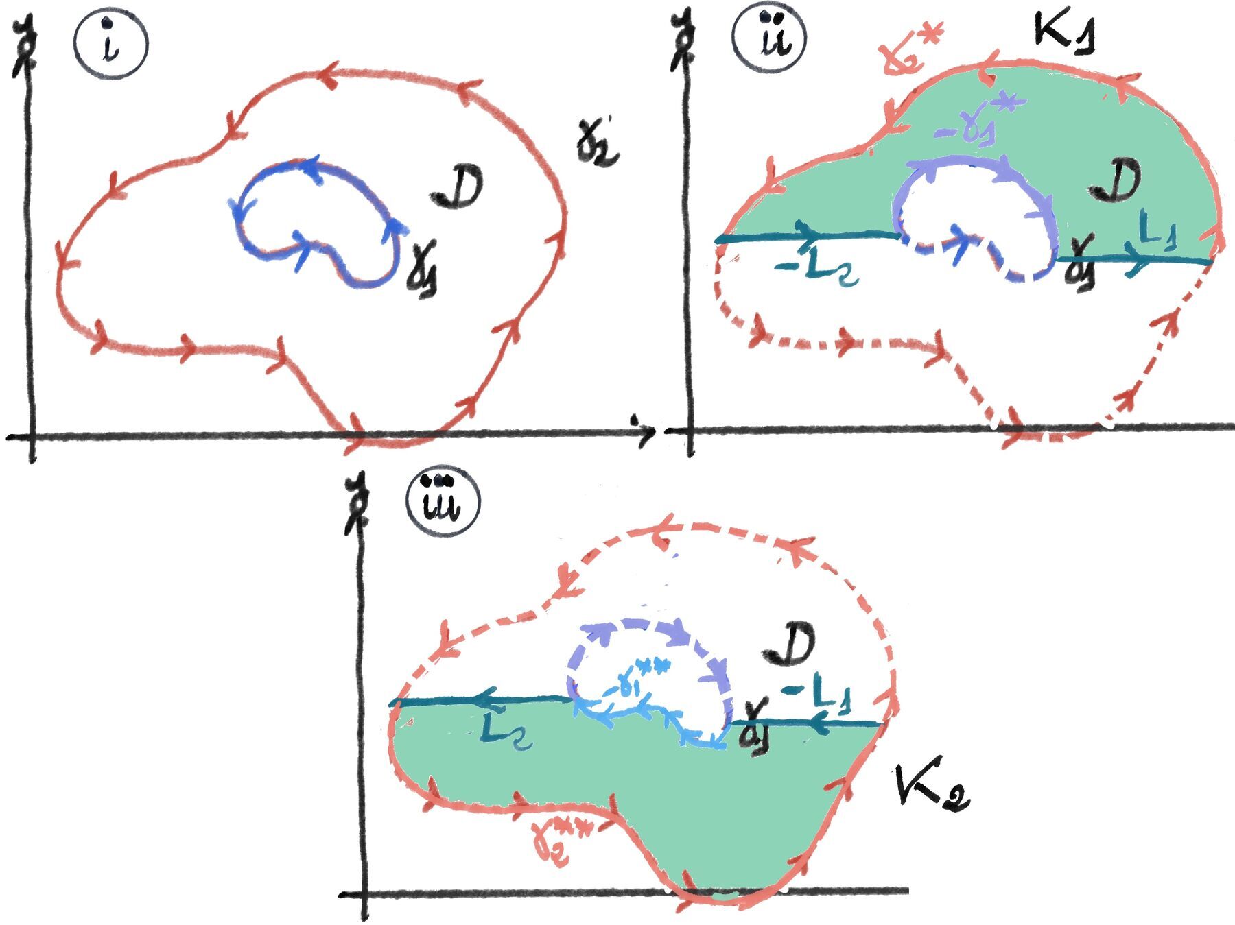
We construct two new, simple closed contours, $K_1$ and $K_2$, that lie entirely within the region G where f(z) is analytic. The direction of integration is essential to ensure $K_1$ and $K_2$ are positively oriented simple closed loops and the regions enclosed by them are simply connected regions (they have no holes) that lie entirely within G.

1. $K_1 = -\gamma_1^* + L_1 + \gamma_2^* - L_2$. It follows $\gamma_1$ backward ($-\gamma_1^*$) from $L_2$ to $L_1$. Then, it crosses the gap via $L_1$ and follows $\gamma_2$ forward ($\gamma_2^*$) from $L_1$ to $L_2$. Finally, it returns via the gap via $L_2$ backward ($-L_2$) (Figure i, ii).
2. $K_2 = -\gamma_1^{**} + L_2 + \gamma_2^{**} - L_1$. It follows $\gamma_1$ backward ($-\gamma_1^{**}$) from $L_1$ to $L_2$. Then, it crosses the gap via $L_2$ and follows $\gamma_2$ forward ($\gamma_2^{**}$) from $L_2$ to $L_1$. Finally, it returns via the gap via $L_1$ backward ($-L_1$) (Figure i, iii).

Since f(z) is analytic throughout G, and since $K_1$ and $K_2$ are simple closed contours lying entirely within a region where f(z) is analytic, we can apply Cauchy’s Theorem (or Cauchy-Goursat): $\oint_{K_1} f(z)dz = \oint_{K_2}f(z)dz = 0$.

Let’s combine the integrals: $\oint_{K_1+K_2} f(z)dz =[\text{By the linearity property of integrals}] \oint_{K_1} f(z)dz + \oint_{K_2} f(z)dz = 0 + 0 = 0$

Substitute the definitions of $K_1$ and $K_2$: $\oint_{K_1+K_2} f(z)dz = \oint_{(-\gamma_1^* + L_1 + \gamma_2^* - L_2)} f(z)dz + \oint_{(-\gamma_1^{**} + L_2 + \gamma_2^{**} - L_1)} f(z)dz = 0$

We group the terms:

$$= \underbrace{\left( \oint_{-\gamma_1^*} f(z)dz + \oint_{-\gamma_1^{**}} f(z)dz \right)}_{-\oint_{\gamma_1} f(z)dz} + \underbrace{\left( \oint_{\gamma_2^*} f(z)dz + \oint_{\gamma_2^{**}} f(z)dz \right)}_{\oint_{\gamma_2} f(z)dz} + \underbrace{\left( \oint_{L_1} f(z)dz + \oint_{-L_1} f(z)dz \right)}_{0} + \underbrace{\left( \oint_{-L_2} f(z)dz + \oint_{L_2} f(z)dz \right)}_{0}$$

• The Cuts Cancel: Since the integral over a segment $L$ is the negative of the integral over the reverse segment $-L$, the integrals along the cuts cancel each other out: $\oint_{L} f(z)dz + \oint_{-L} f(z)dz = 0$
• The $\gamma_1$ and $\gamma_2$ terms combine, e.g., $-\oint_{\gamma_1^*} f(z)dz - \oint_{\gamma_1^{**}} f(z)dz = - \oint_{\gamma_1^* + \gamma_1^{**}} f(z)dz = -\oint_{\gamma_1} f(z)dz$

Hence, $\oint_{K_1+K_2} f(z)dz = -\oint_{\gamma_1} f(z)dz + \oint_{\gamma_2} f(z)dz = 0$. Rearranging the final equation yields the desired result: $\oint_{\gamma_2} f(z)dz = \oint_{\gamma_1} f(z)dz$

Examples

• Calculate the following contour integral: $\oint_\gamma \frac{1}{z²}dz$ where $\gamma$ where $\gamma$ is the rectangle which vertices are -2, -2i, 2, and 2i in the positive orientation (traversed counterclockwise).

The function f(z) = $\frac{1}{z²}$ has a singularity at z = 0, which lies inside γ. We cannot apply Cauchy’s theorem directly. However, we can use the deformation of contours principle.

Let C be a circle of radius 1 centered at the origin (oriented counterclockwise). Since $\frac{1}{z²}$ is not analytic at z = 0 but it is indeed analytic in the annular region between Γ and C (i.e., the region 0 < ∣z∣ < dist(0, γ)), by the deformation of contours principle: $\oint_\gamma \frac{1}{z²}dz = \oint_C \frac{1}{z²}dz$ (Figure i).

The parametric equations of C are: x = cos(t), y = sin(t), 0 ≤ t ≤ 2π. We parametrize the circle C as: z = x + iy = cos(t) + isin(t) = $e^{it} \leadsto dz = ie^{it}dt$.

Now, we compute the integral: $\oint_C \frac{1}{z²}dz = \int_0^{2\pi} \frac{1}{e^{2it}} ie^{it}dt = i \int_0^{2\pi} e^{-it}dt = i \cdot \frac{1}{-i}e^{-it} = - e^{-it}\Big|_{0}^{2\pi} = -e^{-2\pi i} + e^0 = -1 + 1 = 0$

Since $e^{−2πi} = \cos⁡(−2\pi) + i\sin⁡(−2\pi) = 1$.

Therefore: $\boxed{\oint_\gamma \frac{1}{z^2} dz = 0}$

• Calculate $\oint_{\gamma} \frac{e^z}{z²-1}$ where $\gamma$ is the circle centered at the origin with radius 2.

The function f has singularities at z ± 1, both of which lie inside γ, $|z| = 2$ since their magnitudes are 1.

We are going to consider the region inside γ but excluding small circles C₁ and C₂ around z = 1 and z = -1 (oriented clockwise).

By Cauchy’s Integral Theorem for multiply connected regions, the sum of the integral of a function over the contour of a multiply connected region γ traversed counterclockwise is equal to the sum of the integrals over the internal contours (holes) C₁ and C₂, both circles of radius’s length less than one around -1 and 1 respectively and traversed clockwise, $\oint_{\gamma} \frac{e^z}{z²-1} = \oint_{C_1} \frac{e^z}{z²-1} + \oint_{C_2} \frac{e^z}{z²-1}$ (Figure ii)

$\oint_{C_1} \frac{e^z}{z²-1} + \oint_{C_2} \frac{e^z}{z²-1} = \oint_{C_1} \frac{e^z}{z-1}\frac{1}{z+1} + \oint_{C_2} \frac{e^z}{z+1}\frac{e^z}{z-1}$

Cauchy Integral Formula. If a function f is analytic in a simply connected domain D and γ is a simply closed contour (positive orientated) in D. Then, for any point $z_0$ inside γ we have $f(z_0) = \frac{1}{2\pi i}\cdot \int_{\gamma} \frac{f(z)}{z-z_0}dz$

Apply the Cauchy Integral Formula where $f(z) = \frac{e^z}{z-1}, g(z) = \frac{e^z}{z+1} \text{ at } z_0 = -1 \text{ and } 1$ respectively.

$\oint_{C_1} \frac{e^z}{z-1}\frac{1}{z+1} + \oint_{C_2} \frac{e^z}{z+1}\frac{e^z}{z-1} = 2\pi i\frac{e^{-1}}{-2} + 2\pi i\frac{e}{2} = 2\pi i \frac{e-e^{-1}}{2} = \pi i(e-e^{-1})$

Therefore, $\oint_{\gamma} \frac{e^z}{z²-1} = \pi i(e-e^{-1})$