Green's theorem

The excitement of learning separates youth from old age. As long as you’re learning, you’re not old, Rosalyn S.Yalow.

Silence is a source of great strength, Lao Tzu.

Green’s theorem

Green’s theorem relates a line integral around a simple closed curve to a double integral over the plane region R bounded by that curve. If C enclosed a region R counterclockwise, $\vec{F}$ is the vector field defined on the open region containing C defined and differentiable in R, then $\oint_C \vec{F} \cdot{} d\vec{s} = \iint_R curl(\vec{F}) dA ↭ \oint_C Mdx + N dy = \iint_R (N_x-M_y)) dA$

Example. Let C be a circle of radius one center at P(2, 0) counterclockwise. Compute $\oint_C ye^{-x}dx + (\frac{1}{2}x^2-e^{-x})dx.$

Solution.

$\oint_C ye^{-x}dx + (\frac{1}{2}x^2-e^{-x})dx =$[Green’s theorem, $M=ye^{-x}, N=(\frac{1}{2}x^2-e^{-x})$] =$\iint_R curl(\vec{F}) dA = \iint_R (N_x-M_y) dA = \iint_R (x+e^{-x}-e^{-x}) dA = \iint_R x dA = Area(R)\overline {x} = π·2$

Recall that the center of mass of a distribution of mass in space is the unique point at any given time where the weighted relative position of the distributed mass sums to zero, the point where the entire mass of an object may be assumed to be concentrated to visualise its motion, $\overline {x} = \iint_R\frac{1}{Mass}x·δ·dA$ =[If density is one] $\iint_R\frac{1}{Area(R)}xdA$.

Since the circle is symmetric, its center of mass will lie along the x-axis. Therefore, the x-coordinate of the center of mass will be the same as the x-coordinate of the center of the circle (which is 2).

One important consequence of Green’s theorem is that if $\vec{F}$ is defined everywhere in the plane and the curl of a vector field is zero $curl(\vec{F})=0$, then the vector field is conservative, $\oint_C \vec{F} \cdot{} d\vec{r} = \iint_R curl(\vec{F}) dA = \iint_R 0·dA = 0$.

Proof:

First, we are going to prove that $\oint_C Mdx = \iint_R -M_ydA$, this is just a special case when N = 0. A similar argument, $\oint_C Ndy = \iint_R N_xdA$

Futhermore, we will decompose R into simpler, more manageable regions (Figure A). If we can prove that $\oint_{C_1} Mdx = \iint_{R_1} -M_ydA, \oint_{C_2} Mdx = \iint_{R_2} -M_ydA$, the we can add this two statements together and prove the previous result, and that’s true because even though we traverse the edge (the boundary between R₁ and R₂) between the two regions twice, we do so in different orientations, so they cancel each other.

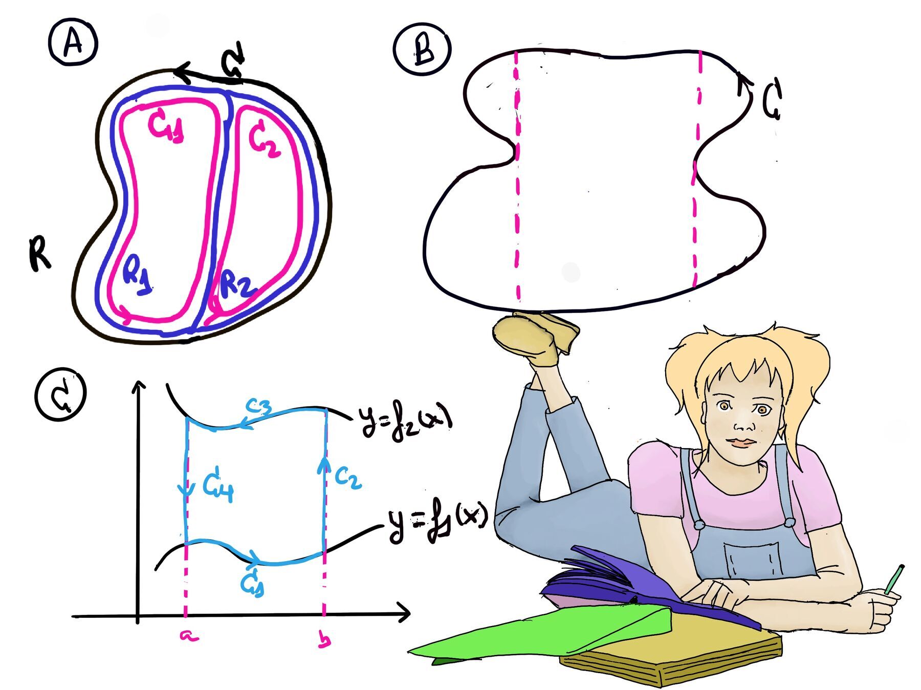
$\oint_C Mdx = \oint_{C_1} Mdx + \oint_{C_2} Mdx = \iint_{R_1} -M_ydA + \iint_{R_2} -M_ydA = \iint_{R} -M_ydA$

Besides, we are going to split the regions between those that have clear boundaries (Figure B) or also referred as vertically simple regions, ∀x: a < x < b, f₁ < x < f₂(x).

Therefore, we only need to prove $\oint_C Mdx = \iint_R -M_ydA$ if R is vertically simple and C is a boundary of R taken counterclockwise. We are going to split the integral into four integrals (Figure C).

$\oint_{C_1} Mdx =$[y = f₁(x), a ≤ x ≤ b] =$\int_{a}^{b} M(x, f_1(x))dx$

$\oint_{C_2} Mdx =$[x = b ⇒ dx = 0] 0, and mutatis mutandis, $\oint_{C_4} Mdx = 0$.

$\oint_{C_3} Mdx =$[y = f₂(x), b ≤ x ≤ a] =$\int_{b}^{a} M(x, f_2(x))dx = -\int_{a}^{b} M(x, f_2(x))dx$

Putting all together, $\oint_C Mdx = \oint_{C_1} Mdx + \oint_{C_2} Mdx + \oint_{C_3} Mdx + \oint_{C_4} Mdx = \int_{a}^{b} M(x, f_1(x))dx -\int_{a}^{b} M(x, f_2(x))dx = \int_{a}^{b} M(x, f_1(x)-f_2(x))dx$

On the other side of the equation, $\iint_{R} -M_ydA = -\int_{a}^{b}(\int_{f_1(x)}^{f_2(x)} \frac{∂M}{∂y}dy)dx$

The inner integral is $\int_{f_1(x)}^{f_2(x)} \frac{∂M}{∂y}dy = M(x, f_2(x))-M(x, f_1(x))$

$\iint_{R} -M_ydA = -\int_{a}^{b}(\int_{f_1(x)}^{f_2(x)} \frac{∂M}{∂y}dy)dx = -\int_{a}^{b} (M(x, f_2(x))-M(x, f_1(x)))dx$ ⇒ $\oint_C Mdx = \iint_R -M_ydA$ ∎

Bibliography

1. NPTEL-NOC IITM, Introduction to Galois Theory.
2. Algebra, Second Edition, by Michael Artin.
3. LibreTexts, Calculus. Abstract and Geometric Algebra, Abstract Algebra: Theory and Applications (Judson).
4. Field and Galois Theory, by Patrick Morandi. Springer.
5. Michael Penn, Andrew Misseldine, blackpenredpen, and MathMajor, YouTube’s channels.
6. Contemporary Abstract Algebra, Joseph, A. Gallian.
7. MIT OpenCourseWare, 18.01 Single Variable Calculus, Fall 2007 and 18.02 Multivariable Calculus, Fall 2007, YouTube.
8. Calculus Early Transcendentals: Differential & Multi-Variable Calculus for Social Sciences.