Surface Integrals of Vector Fields. Flux.

One who asks a question is a fool for a minute; one who does not remains a fool forever, Chinese proverb

Flux

A line integral gives us the ability to integrate multivariable functions and vector fields over arbitrary curves in a plane or in space.

Flux is another line integral, more precisely, the flux of a vector field $\vec{F}$ across a curve C is defined as the dot product of the vector field and the unit normal vector n to the surface S, that is, $\oint_{C} \vec{F}·\vec{n}·ds$ where $\vec{n}$ is the unit normal vector to the curve C (perpendicular to the curve and has length 1) pointing 90° in clockwise direction and ds represents an infinitesimal area element on the surface S (Figure 1).

If we break the curve C into small pieces Δs, flux = $\lim_{\Delta s \to 0} (\sum \vec{F}·\vec{n}·ΔS)$.

Recall that work = $\oint_{C} \vec{F}·d\vec{r} = \oint_{C} \vec{F}·\hat{\mathbf{T}}·ds$, i.e., the dot product of the vector field with the unit tangential vector (in the direction of motion) with respect to the curve. I am loosely speaking summing the tangential component of $\vec{F}$ along the curve C. It measures when I move along the curve how much I am going with or against $\vec{F}$.

On the other hand, flux measures when I move along the curve how much the field is going across the curve. I am loosely speaking summing the normal component of $\vec{F}$ along the curve C.

It represents the amount of a vector field (let’s think about it as a vector field) passing through a surface. If the field is a flow of water, for example, the flux measures how much fluid passes through the curve C per unit time or represents the volume of water flowing through the surface per unit time. It refers to the amount of fluid, energy, or other quantity that flows through a curve in a given direction per unit time.

To be more precise, what flows across C from left-to-right is counted positively, and right-to-left is counted negatively, so in fact, it is the net flow per unit time.

Observe Figure 2 and 3 (2 rotated), we are zooming over a little piece of my curve C (length ΔS) and a fluid flows to the right. How much fluid, energy or whatever passes through this piece of my curve over time. It is a parallelogram with Area = base · height = $ΔS· (\vec{F}·\vec{n})$

• Example. C is a circle of radius a at origin counterclockwise $\vec{F} = x\vec{i}+y\vec{j}$ -a field that is pointing radially away from the origin- (Figure 4)

Solution.

$\vec{F}||\vec{n} ⇒ \vec{F}·\vec{n} = |\vec{F}|·|\vec{n}|·cos(0) = |\vec{F}|·1·1 = |\vec{F}|$ =[Across the circle] a ⇒$\int_{C} \vec{F}·\vec{n}·ds = \int_{C} a·ds = a·\int_{C} ds = a·length(C) = a·2πa = 2πa^2.$

• Example. C is a circle of radius a at origin counterclockwise $\vec{F} = -y\vec{i}+x\vec{j}$ -a field that is defined counterclockwise around the origin- (Figure A)

$\vec{F} ⊥ \vec{n} ⇒ \vec{F}·\vec{n} = |\vec{F}|·|\vec{n}|·cos(0) = |\vec{F}|·1·0 = 0⇒ \int_{C} \vec{F}·\vec{n}·ds = 0$

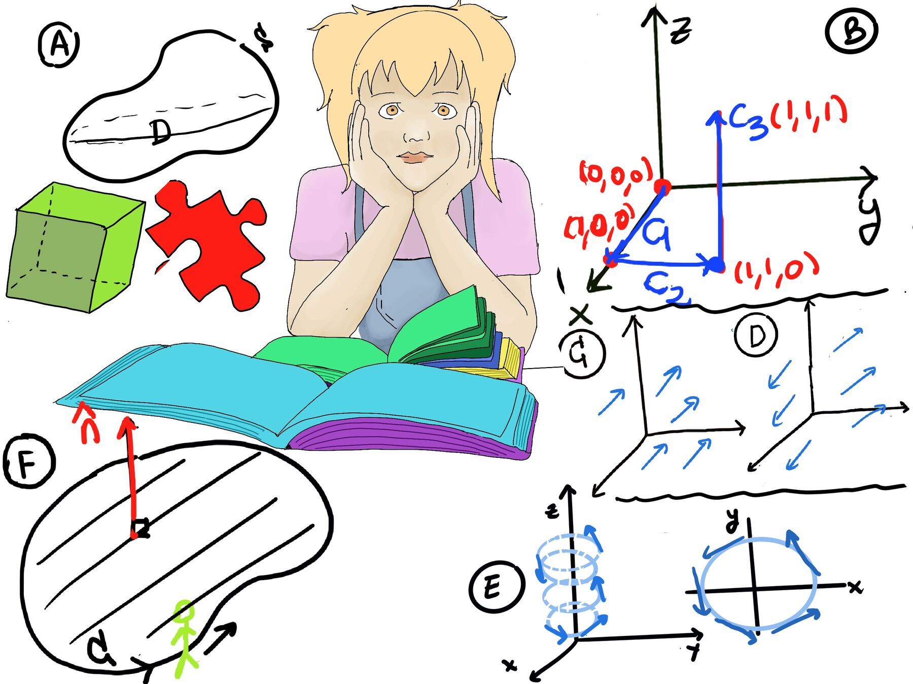
The next question to resolve is how we do the calculation using components. Remember that $d\vec{r} = \hat{\mathbf{T}}·ds = ⟨dx, dy⟩$. Since $\vec{n}~\text{is}~\hat{\mathbf{T}}$ rotated 90° clockwise, $\vec{n}ds = ⟨dy, -dx⟩$ (Figure B).

Therefore, if $\vec{F} = ⟨P, Q⟩$, then $\int_{C} \vec{F}·\vec{n}·ds = \int_{C} ⟨P, Q⟩·⟨dy, -dx⟩ = \int_{C} -Qdx + Pdy.$

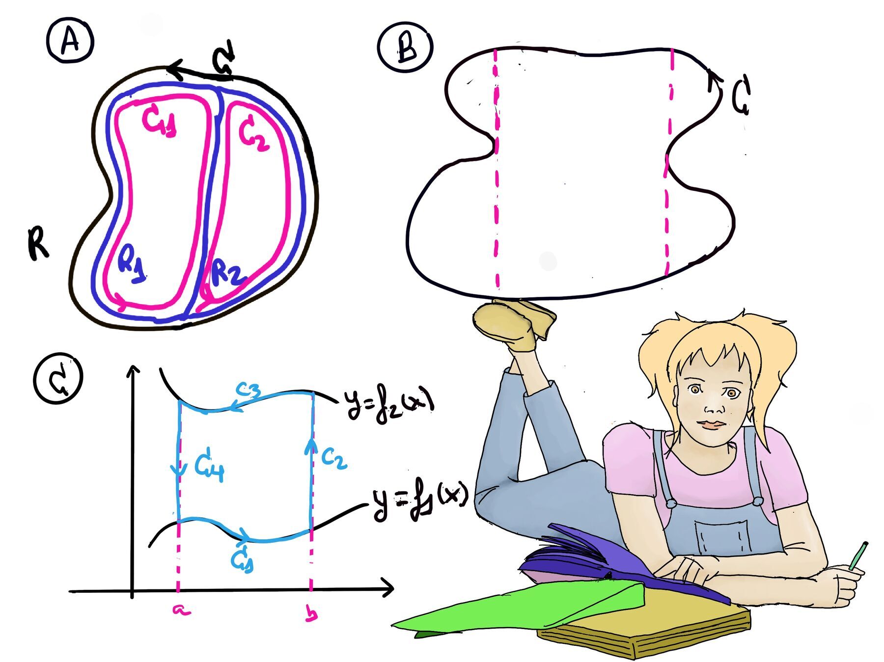
Green’s Theorem for Flux relates the flux of a vector field across a closed curve to the circulation of the vector field around the curve. It states that if C encloses a region R counterclockwise and $\vec{F} = ⟨P, Q⟩$ is defined on R, then $\oint_C \vec{F} \vec{n}·d\vec{s} = \int \int_{R} div \vec{F}dA$ where $div \vec{F} = P_x + Q_y.$

We can interpret $\oint_C \vec{F}·\vec{n}·d\vec{s}$ (Figure C) as the flux of the vector field out of R through C.

Proof.

We want to prove $\oint_C \vec{F} \vec{n}·d\vec{s} = \int \int_{R} div \vec{F}dA ↭ \oint_C -Qdx + Pdy = \int \int_{R} (P_x + Q_y)dA$.

Let’s rename -Q = M, P = N ⇒ By Green’s Theorem, $\oint_C \vec{F}·\vec{n}·d\vec{s} = \oint_C Mdx + Ndy = \int \int_{R} (N_x-M_y)dA = \int \int_{R} (P_x+Q_y)dA$ ∎

Observe that one compute the force done across the closed curve, but this one computes the vector field out of the region.

• Example. C is a circle of radius a at origin counterclockwise $\vec{F} = x\vec{i}+y\vec{j}$ -a field that is pointing radially away from the origin- (Figure 4)

$\vec{F} = ⟨P, Q⟩, div \vec{F} = P_x + Q_y = \frac{∂}{∂x}(x)+\frac{∂}{∂y}(y) = 1 + 1 = 2.$

$\oint_C \vec{F} \vec{n}·d\vec{s} = \int \int_{R} div \vec{F}dA = \int \int_{R} 2dA = 2\int \int_{R} dA = 2area(R) = 2πa^2$

The divergence of a vector field simply measures how much the flow is expanding at a given point or the amount of fluid added to the system per unit time and area.

Both version of Green theorems, $\oint_{C} \vec{F}·\vec{n}·ds = \int \int_R div\vec{F}dA \text{and} \oint_C \vec{F}·\hat{\mathbf{T}}·ds = \int \int_R curl\vec{F}dA$ only work when the vector field ($\vec{F}$) is defined everywhere in R.

Example. $\vec{F} = \frac{-y\vec{i}+x\vec{j}}{x^2+y^2}, \vec{F}$ is not defined at the origin, everywhere else $curl(\vec{F}) = 0$

There are situations as illustrated in Figure D where we can not use Green theorems directly.

And yet, Figure A, $\oint_{C’} \vec{F}d\vec{r}-\oint_{C’’} \vec{F}d\vec{r} = \int \int_R curl \vec{F}dA$

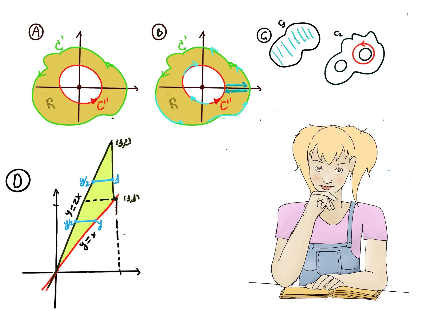
Observe, Figure B, that we can create a curve that will enclose this region counterclockwise, hence the total line integral $\oint_C \vec{F}·\hat{\mathbf{T}}·ds = \oint_{C’} -\oint_{C’’}$[They are in different directions, that’s why it is negative and there are two border segments that cancel out -draw in darker color to help the reader see it-] = $\int \int_R curl \vec{F}dA$

Definition. A connected region R in the plane is simply connected if the interior of any close curve in A is also contained in R, that is, the region A does not have holes in it (Figure C), C₁ is simply connected and C₂ is not simply connected (Observe the curve in red).

It is important because if a vector field is defined everywhere in a connected region, you don’t need to worry about Green’s Theorem. More formally, if the domain where $\vec{F}$ is defined (and differentiable) is simply connected, then we can always apply the Green’s theorem. In our previous example, our domain was not simply connected.

Recall our criteria, if a curl of the vector field is zero and defined in the entire plane, then the vector field is conservative (a gradient field) ↭ $curl \vec{F}=0$ and domain where $vec{F}$ is defined is simply connected, then $\vec{F}$ is conservative ($\oint_C \vec{F}·\hat{\mathbf{T}}·ds = \int \int_R curl\vec{F}dA = \int \int_R 0·dA$ = 0) -C is a closed curve obviously-.

How we can set it up to swap or exchange the integrals, $\int_{0}^{1}\int_{x}^{2x} fdydx$ (Figure D).

$\int_{0}^{1}\int_{x}^{2x} fdydx = \int_{0}^{1}\int_{\frac{y}{2}}^{y} fdxdy + \int_{1}^{2}\int_{\frac{y}{2}}^{1} fdxdy$

Bibliography

1. NPTEL-NOC IITM, Introduction to Galois Theory.
2. Algebra, Second Edition, by Michael Artin.
3. LibreTexts, Calculus and Calculus 3e (Apex). Abstract and Geometric Algebra, Abstract Algebra: Theory and Applications (Judson).
4. Field and Galois Theory, by Patrick Morandi. Springer.
5. Michael Penn, and MathMajor.
6. Contemporary Abstract Algebra, Joseph, A. Gallian.
7. YouTube’s Andrew Misseldine: Calculus. College Algebra and Abstract Algebra.
8. MIT OpenCourseWare 18.01 Single Variable Calculus, Fall 2007 and 18.02 Multivariable Calculus, Fall 2007.
9. Calculus Early Transcendentals: Differential & Multi-Variable Calculus for Social Sciences.