The Divergence Theorem

Sixth rule A, Almost all properties apply to the empty set, most of them to finite sets, and dividing by zero is a terrible idea. 0 is not a number, 1 plus one equals zero in ℤ₂ and $\sqrt{2}$ and $-\sqrt{2}$ are algebraically the same. Galois’ Theory and Partial differential equations are not for the faint of heart. Absolute numbers have no meaning, Apocalypse, Anawim, #justtothepoint.

The Divergence Theorem

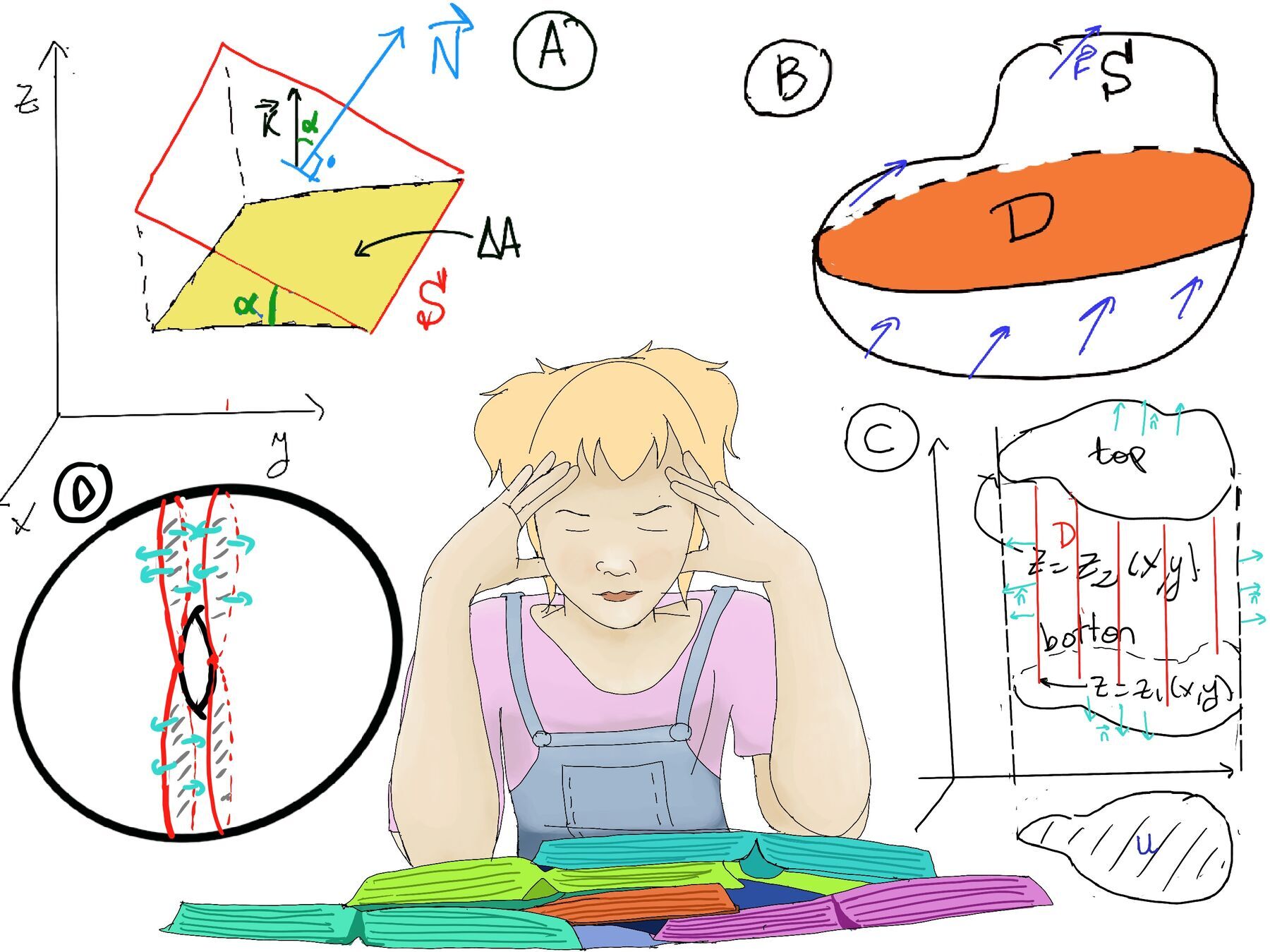
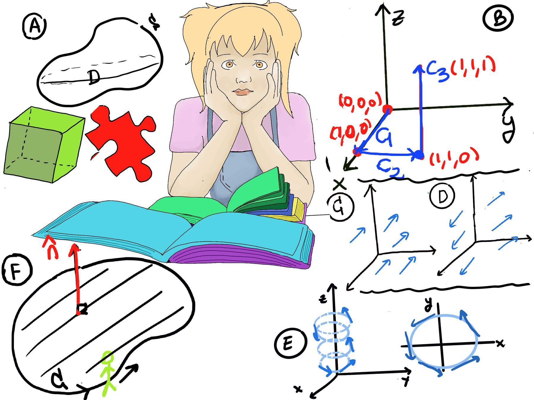
The divergence theorem, also known as Gauss’s or Gauss-Green theorem, is a fundamental result that relates the flux of a vector field through a closed surface S enclosing a region D, $\vec{F}$ defined and differentiable everywhere in D, orientated with $\hat{\mathbf{n}}$ outwards, to the divergence of the vector field within the region enclosed by the surface (Figure B).

Divergence Theorem. Let D be a region in three-dimensional space bounded by a closed surface S with outward unit normal vector $\hat{\mathbf{n}}$. If $\vec{F}$ is a vector field defined on an open region containing D, then the outward flux of $\vec{F}$ across S is given by the triple integral of the divergence of F over the region D: $\oint_S \vec{F} \cdot d\vec{S} = \int \int \int_{D} div \vec{F} dV$

Let $\vec{F} = P\vec{i} + Q\vec{j} + R\vec{k}, div(\vec{F}) = P_x +Q_y + R_z.$

In our previous example, we calculate that the flux of $\vec{F}= z\hat{\mathbf{k}}$ through a sphere of radius a was $\frac{4}{3}πa^3.$

By using Divergence Theorem, we know that $\oint_S \vec{F} \cdot d\vec{S} =\int \int_{S} \vec{F}·\hat{\mathbf{n}}·dS = \int \int_{S} z·\hat{\mathbf{k}}·\hat{\mathbf{n}}·dS = \int \int \int_{D} div(z·\hat{\mathbf{k}}) dV$ =[$ div(\vec{F}) = P_x +Q_y + R_z = 0 + 0 + 1 = 1$] $\int \int \int_{D} dV = vol(D) = \frac{4}{3}πa^3.$

Physical Interpretation.

The divergence of a vector field $\vec{F}$ represents the tendency of the field to flow away or expand things, the source rate or amount of flux generated per unit volume. If you have an incompressible fluid flow (given mass occupied a fixed volume) with velocity given by our vector

The divergence theorem states that $\oint_S \vec{F} \cdot d\vec{S} =\int \int_{S} \vec{F}·\hat{\mathbf{n}}·dS$ the flux of a vector field through a closed surface enclosing a region represents the total amount of stuff that goes out of the region per unit time (the net flow of the vector field or how much fluid is passing through this surface or leaving the region D per unit time) -the left side of the equation- equals the total amount of sources minus the sinks of the field within the enclosed region.

$\oint_S \vec{F} \cdot d\vec{S} = \int \int \int_{D} div \vec{F} dV$. Using components, $\oint_S ⟨P, Q, R⟩·\hat{\mathbf{n}}·dS = \int \int \int_{D} (P_x+Q_y+R_z)dV$

Notation. The ∇ operator, often referred to as “del” or “nabla”, is a vector differential operator used in vector calculus to express various mathematical operations involving differentiation and gradients, $∇ = ⟨\frac{∂}{∂x}, \frac{∂}{∂y}, \frac{∂}{∂z}⟩, ∇f = ⟨\frac{∂f}{∂x}, \frac{∂f}{∂y}, \frac{∂f}{∂z}⟩$, and more importantly, $∇·\vec{F} =⟨\frac{∂}{∂x}, \frac{∂}{∂y}, \frac{∂}{∂z}⟩·⟨P, Q, R⟩ = \frac{∂P}{∂x} + \frac{∂Q}{∂y} + \frac{∂R}{∂z} = div(\vec{F})$

Proof.

First, we are going to prove that $\oint_S ⟨0, 0, R⟩·\hat{\mathbf{n}}·dS = \int \int \int_{D} R_zdV$, then we can get the general case by summing one of such identities, one for each component, hence $\oint_S \vec{F} \cdot d\vec{S} = \oint_S ⟨P, Q, R⟩·\hat{\mathbf{n}}dS = \int \int \int_{D} div \vec{F} dV = \int \int \int_{D} (P_x+Q_y+R_z)dV$

If the region is vertically simple, that is, bounded on the left and right by vertical lines and bounded on the top and bottom by function of x and y, z = z₁(x, y), z = z_s(x, y) (Figure C)

Let’s consider the right-hand side of the equation,

$\int \int \int_{D} R_zdV = \int \int_{U} (\int_{z_1(x, y)}^{z_2(x, y)} R_zdz)dxdy = \int \int_{U} (R(x, y, z_2(x, y)-R(x, y, z_1(x, y))))dxdy$ 🚀

Let’s consider the left-hand side of the equation,

$\oint_S ⟨0, 0, R⟩·\hat{\mathbf{n}}·dS = \oint_{SBottom} ⟨0, 0, R⟩·\hat{\mathbf{n}}·dS + \oint_{Stop} ⟨0, 0, R⟩·\hat{\mathbf{n}}·dS + \oint_{SSides} ⟨0, 0, R⟩·\hat{\mathbf{n}}·dS$ [Recall that we have seen that we can compute $\hat{\mathbf{n}}·dS$ when it is in a graph z = z₂(x, y), $\hat{\mathbf{n}}·dS = ⟨-\frac{∂z_2}{∂x}, -\frac{∂z_2}{∂y}, 1⟩dxdy$]

$\oint_{Stop} ⟨0, 0, R⟩·\hat{\mathbf{n}}·dS = \oint_{Stop} ⟨0, 0, R⟩·⟨-\frac{∂z_2}{∂x}, -\frac{∂z_2}{∂y}, 1⟩dxdy = \oint_{Stop} Rdxdy = \int \int_{U} R(x, y, z_2(x, y))dxdy$

Mutates Mutandis, when we want to compute the button, $\hat{\mathbf{n}}·dS = ⟨+\frac{∂z_1}{∂x}, +\frac{∂z_1}{∂y}, -1⟩dxdy$ and this is so because we have established that $\hat{\mathbf{n}}$ is orientated upwards.

$\oint_{SBottom} ⟨0, 0, R⟩·\hat{\mathbf{n}}·dS = \oint_{Stop} ⟨0, 0, R⟩·⟨\frac{∂z_2}{∂x}, \frac{∂z_2}{∂y}, -1⟩dxdy = \oint_{Stop} Rdxdy = \int \int_{U} -R(x, y, z_1(x, y))dxdy$

$\oint_{SSides} ⟨0, 0, R⟩·\hat{\mathbf{n}}·dS = 0$ because ⟨0, 0. R⟩ is tangent to the sides, so flux through the sides is zero.

$\oint_S ⟨0, 0, R⟩·\hat{\mathbf{n}}·dS = \oint_{SBottom} ⟨0, 0, R⟩·\hat{\mathbf{n}}·dS + \oint_{Stop} ⟨0, 0, R⟩·\hat{\mathbf{n}}·dS + \oint_{SSides} ⟨0, 0, R⟩·\hat{\mathbf{n}}·dS = \int \int_{U} (R(x, y, z_2(x, y)-R(x, y, z_1(x, y))))dxdy$ 🚀

If D is not vertically simple, we can decompose it into simple pieces (Figure D), and the regions shared by these pieces are cancelled out because $\hat{\mathbf{n}}$ has opposite orientations.

The diffusion equation

It describes how quantities such as heat, mass, or charge distribute over time in a medium where they are free to move. It describes the process of diffusion, which is the spontaneous movement of particles or substances as they spread out from regions of high concentration to regions of low concentration, e.g., the motion of smoke in air, dye in a solution, etc.

Let u be the concentration at a given point P(x, y, z), u = u(x, y, z). The diffusion equation can be expressed as $\frac{∂u}{∂t} = k·∇^2u$ where k is the diffusion coefficient (a constant) and ∇^2u is called the Laplacian (div) = ∇·∇u, that is, the divergence of gradient.

$\frac{∂u}{∂t} = k∇^2u = k∇·∇u = k(\frac{∂^2u}{∂x^2}+\frac{∂^2u}{∂y^2}+\frac{∂^2u}{∂z^2})$. It is also know as the heat equation.

It was first developed by Joseph Fourier in 1822 for the purpose of modeling how a quantity such as heat diffuses through a given region where u is the temperature.

Let $\vec{F}$ be the flow of the smoke, its direction is telling me in which direction the smoke is moving, and its magnitude indicates what amount is moving and how fast is moving. Mere observation tell us that the smoke will flow from high concentration towards low concentration areas. In other words, $\vec{F}$ is directed along ∇u, $\vec{F}$ is proportional to -∇u. In fact, $\vec{F} = -k∇u$ (🚀)

We want to know $\frac{∂u}{∂t}$. Let’s calculate the flux out of D through a region S: (Figure A)

$\oint_S \vec{F} \cdot d\vec{S}$ is the amount of smoke through S per unit time. I can also compute it by looking at the total amount of smoke in the region and seeing how much it changes and that is mathematically the derivate with respect to t (time) of the total amount of smoke in the region $-\frac{d}{dt}(\int \int \int_{D} udV)$ (it is negative because we are counting the amount of smoke that we are losing.)

By the Divergence Theorem we know that

$\oint_S \vec{F} \cdot d\vec{S} = \oint_S \vec{F} ·\hat{\mathbf{n}}·dS = \int \int \int_{D} div(\vec{F})dV = -\frac{d}{dt}(\int \int \int_{D} udV) = -\int \int \int_{D} \frac{∂u}{∂t}dV$ Basically, the idea behind the last step is that $\frac{d}{dt} (\sum_{i} u(x_i,y_i,z_i,t)ΔV_i) = \sum_{i} \frac{∂u}{∂t}(x_i,y_i,z_i,t)ΔV_i$.

Notice that $\int \int \int_{D} div(\vec{F})dV = -\int \int \int_{D} \frac{∂u}{∂t}dV ⇒ \frac{1}{vol(D)}\int \int \int_{D} div(\vec{F})dV = \frac{1}{vol(D)}\int \int \int_{D} -\frac{∂u}{∂t}dV$. In words, the average of $div(\vec{F})$ in D is equal to the average of $-\frac{∂u}{∂t}$ in any region D of V ⇒$div(\vec{F}) = -\frac{∂u}{∂t}$

$\frac{∂u}{∂t} = -div(\vec{F}) =$[🚀] $kdiv(∇u) = k∇^2u ⇒ \frac{∂u}{∂t} = k∇^2u,$ and that’s how we got the diffusion equation.

Bibliography

1. NPTEL-NOC IITM, Introduction to Galois Theory.
2. Algebra, Second Edition, by Michael Artin.
3. LibreTexts Mathematics, Calculus and Calculus 3e (Apex). Abstract and Geometric Algebra, Abstract Algebra: Theory and Applications (Judson).
4. Field and Galois Theory, by Patrick Morandi. Springer.
5. Michael Penn, and MathMajor.
6. Contemporary Abstract Algebra, Joseph, A. Gallian.
7. YouTube’s Andrew Misseldine: Calculus. College Algebra and Abstract Algebra.
8. MIT OpenCourseWare 18.01 Single Variable Calculus, Fall 2007 and 18.02 Multivariable Calculus, Fall 2007.
9. Calculus Early Transcendentals: Differential & Multi-Variable Calculus for Social Sciences.